Free Courses

[Solution]

Introduction

In the rapidly evolving landscape of safety-critical software development, integrating modern tools can significantly enhance productivity and flexibility. Ansys SCADE, renowned for its robust support in developing certified software, can be further empowered by leveraging Jupyter Notebooks.

This article explores how Jupyter Notebooks can extend SCADE’s capabilities, enabling developers to streamline workflows, automate tasks, and enhance data visualization. Discover how this synergy can revolutionize your development process.

Photo credit: Pixabay @ Pexels

A first-order low-pass filter example

In this article, we’ll demonstrate how to extend SCADE’s capabilities using a simple yet effective example: a first-order low-pass filter.

We will use the following recursive equation to represent our RC Filter:

$$y[i]= y[i-1] + a(x[i] – y[i-1])$$

Where:

$$\alpha = \frac{\Delta t}{\frac{1}{2 \pi \omega_{c}}+ \Delta t}$$

$\Delta t$ is the interval between each sampling

$\omega_{c}$ is the cutoff frequency

Designing our filter in SCADE

Implementing a first order low pass filter in SCADE is quite simple and would give the following diagram:

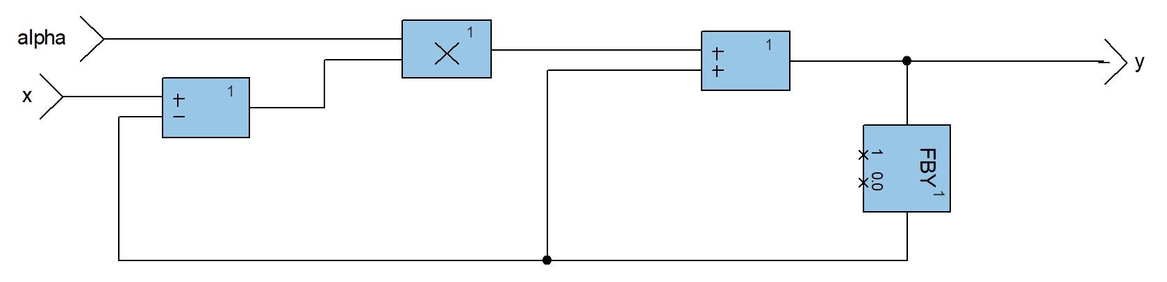
Low Pass filter in SCADE

Note the use of the FBY operator, which allows us to reference the value of y from previous cycles ($y[i-1]$ in our equation above).

Planning our tests

Testing a low-pass filter involves verifying its performance against expected behavior, such as attenuation of high-frequency components and preservation of low-frequency components. We will perform two kinds of tests to validate our filter.

Time-domain testing

Test with step inputs to measure settling time, overshoot, and response characteristics.

Frequency response testing

Verify the filter’s behavior across a range of frequencies:

• Test the filter with low and high-frequency sine waves to observe attenuation, or frequency sweeps (sinusoids of varying frequencies).
• Compare output magnitudes against the theoretical response (e.g., -3 dB at cutoff frequency for a first-order filter).
• Visualize the frequency response using a Fast Fourier Transform or a Bode plot:
  • Cutoff frequency: verify that the filter attenuates signals beyond the designed cutoff frequency.
  • Phase shift: check the phase delay introduced by the filter, especially for critical applications.
  • Attenuation rate: measure how quickly the filter reduces unwanted frequencies.

Testing our filter in SCADE

Time-domain testing

We design a test harness in SCADE to generate the step signal:

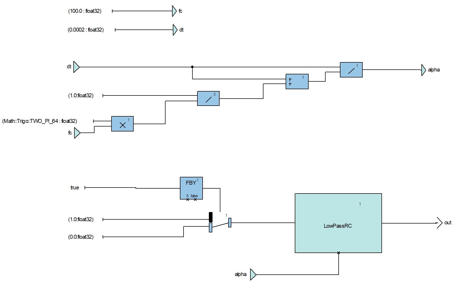
Step harness

Note that we could also use a test scenario that leverages files of pre-calculated input values and expected output values.

This test harness is executed in the SCADE simulator. We can observe the response values on simple graphs:

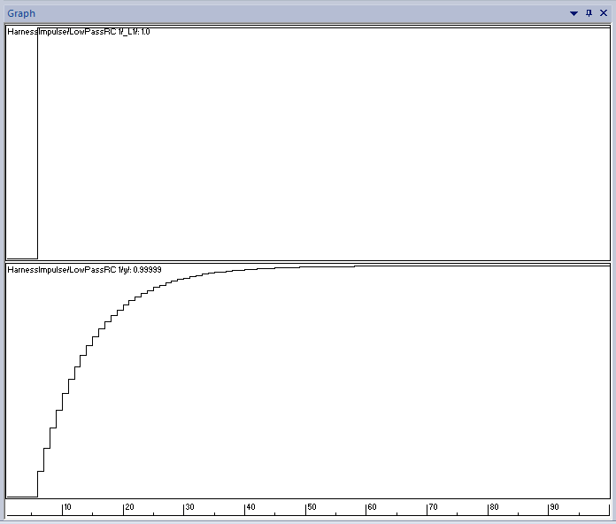
Step response in SCADE

Frequency response testing

We create a new test harness to generate a sine wave signal:

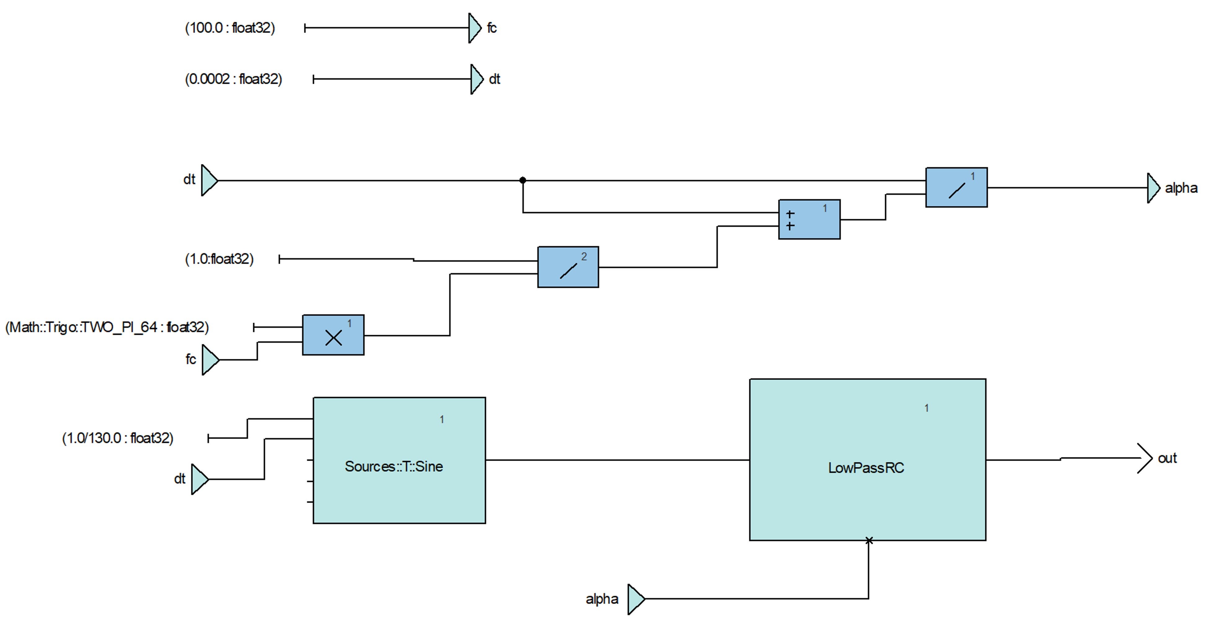
Sine wave signal harness

Using the simulator, we can plot the input and output signals:

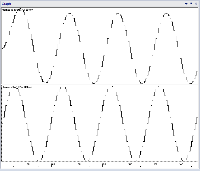
Sine wave signal and filtered signal

This gives us a first view of our filter’s output. However, SCADE is a software development tool and is not suited for more detailed signal analysis. We need a different set of tools to verify the frequency response of our filter.

To go further, we will rely on a tool called the SCADE Python Wrapper: it provides a Python proxy to the generated C code from a SCADE Suite application. This allows us to run our SCADE application directly from Python code, set inputs, observe local variables, outputs, and probes.

This opens the entire Python ecosystem to a SCADE application.

Testing our filter with a Jupyter notebook

To test our filter further, we will use a Jupyter notebook in which we will exercise our SCADE model.

Installing the SCADE Python Wrapper

First, let’s install the SCADE Python Wrapper. It is available as a public Python package which can be installed from the Ansys SCADE Extension Manager (in SCADE 2024R2+), or from a simple command line in the included Python installation:

pip install ansys-scade-python-wrapper

Generating a Python module for our SCADE model

Once the Python wrapper is installed for our instance of SCADE, we see new screens and options in our SCADE code generation settings.

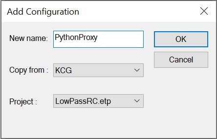
We start by creating a new code generation configuration under Project > Configurations:

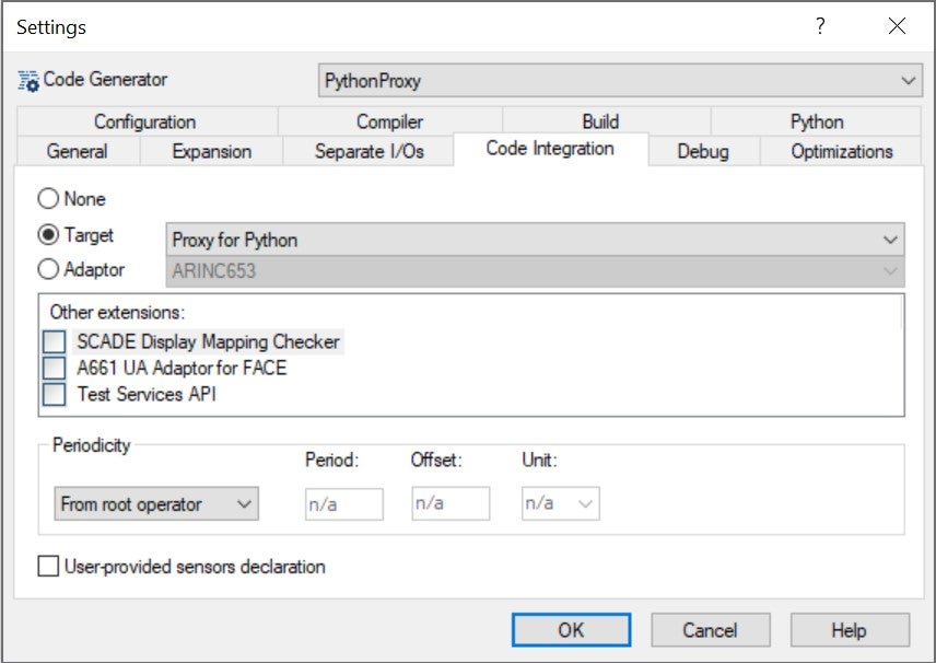
Then, in Project > Code Generator > Settings > Code Integration, we select Proxy for Python as a Target:

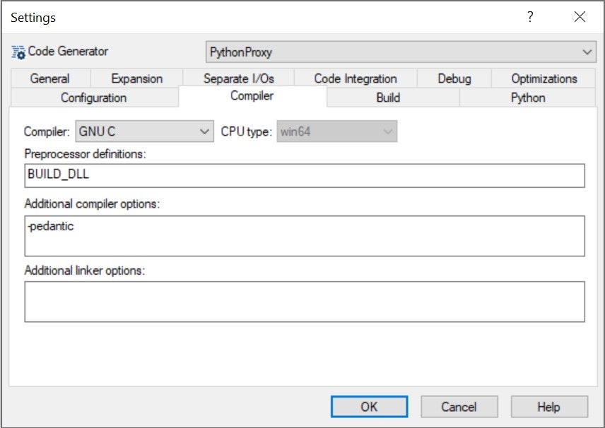
We select, in tab Compiler, the proper options for our target environment:

In tab General, we check that the proper root operator is selected:

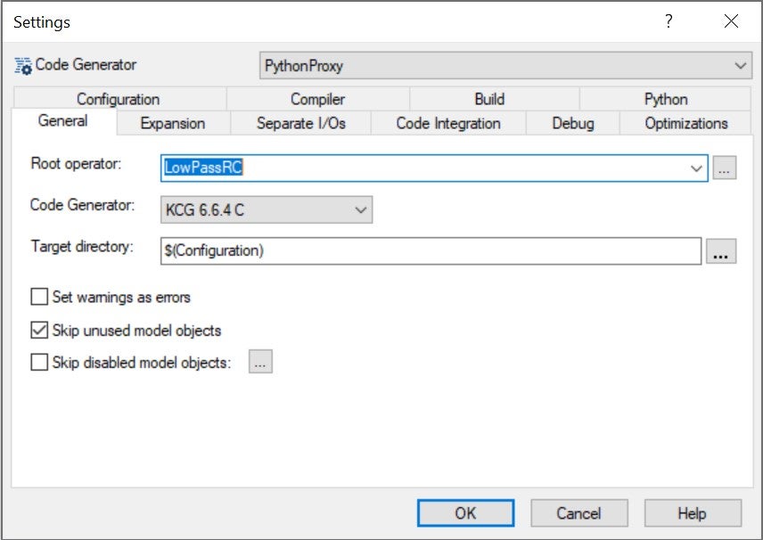
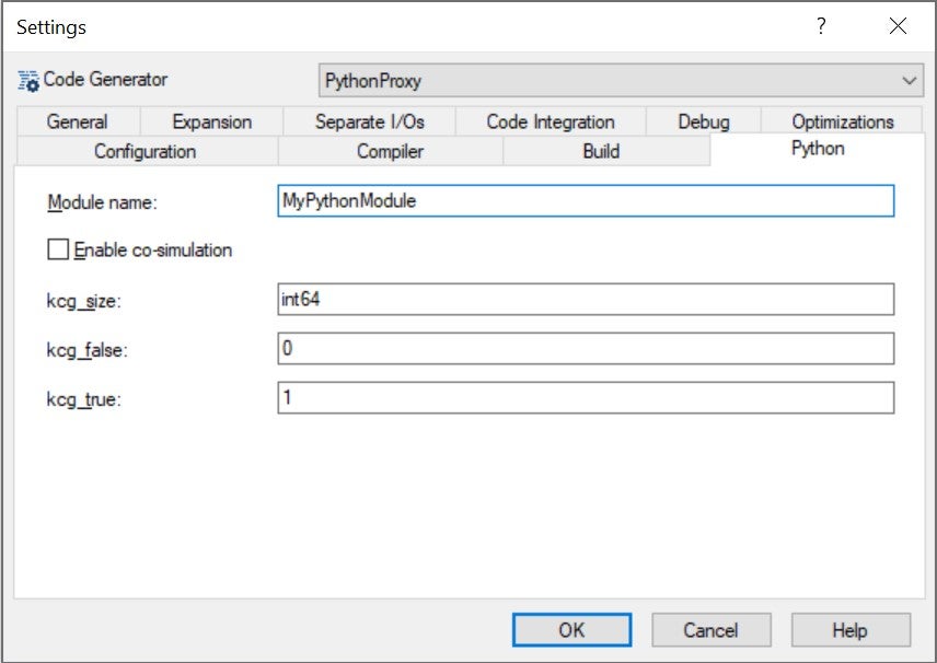
Finally, in tab Python, we choose a module name:

We now generate and build the module, which ends up in the target directory (as previously defined in code generator options). Two important files are generated: MyPythonModule.py and MyPythonModule.dll.

MyPythonModule.py uses ctypes to wrap our operator in a class that exposes its inputs (x and alpha), its output (y), and functions to run it:

# generated by SCADE Python Proxy Extension 1.8.2

from pathlib import Path
import ctypes

# load the SCADE executable code
_lib = ctypes.cdll.LoadLibrary(str(Path(__file__).with_suffix('')))

# C structures
class _CinC_LowPassRC(ctypes.Structure):
    _fields_ = [('x', ctypes.c_float),
                ('alpha', ctypes.c_float)]

class LowPassRC:
    def __init__(self, cosim: bool = True):
        self._in_c = _CinC_LowPassRC()
        alloc_fct = _lib.py_alloc_LowPassRC
        alloc_fct.argtypes = []
        alloc_fct.restype = ctypes.c_void_p
        context = alloc_fct()
        self._out_c = ctypes.c_void_p.from_address(context)
        offsets = (ctypes.c_int64 * 1).in_dll(_lib, "py_offsets_LowPassRC")
        self.reset_fct = _lib.LowPassRC_reset
        self.reset_fct.restype = ctypes.c_void_p
        self.cycle_fct = _lib.LowPassRC
        self.cycle_fct.argtypes = [
            ctypes.POINTER(_CinC_LowPassRC),
            ctypes.POINTER(ctypes.c_void_p),
        ]
        self.cycle_fct.restype = ctypes.c_void_p
        self._y = ctypes.c_float.from_address(context + offsets[0])

    def __del__(self):
        free_fct = _lib.py_free_LowPassRC
        free_fct.argtypes = [ctypes.c_void_p]
        free_fct.restype = None
        free_fct(ctypes.byref(self._out_c))

    def call_reset(self) -> None:
        self.reset_fct(ctypes.byref(self._out_c))

    def call_cycle(self, cycles: int = 1, refresh: bool = True, debug: bool = False) -> None:
        for i in range(cycles):
            self.cycle_fct(
                self._in_c,
                self._out_c,
            )

    @property
    def x(self) -> float:
        return self._in_c.x

    @x.setter
    def x(self, value: float) -> None:
        self._in_c.x = value

    @property
    def alpha(self) -> float:
        return self._in_c.alpha

    @alpha.setter
    def alpha(self, value: float) -> None:
        self._in_c.alpha = value

    @property
    def y(self) -> float:
        return self._y.value

# end of file

Setting up our Jupyter notebook

Jupyter notebooks are a great tool for interactive programming. They allow a developer to write code and documentation in successive blocks that can then be re-run at will. The notebook presented in this article is available for download at the end. For now, let’s walk through it section by section.

First, we initiate the notebook by adding the generated Python Proxy module to our path and importing it. The most straightforward way to do this would be to append it to sys.path:

import sys, os

harness_dir = os.path.join(os.path.abspath(''), 'LowPassRCSuite', 'PythonProxy')
sys.path.append(harness_dir)
from MyPythonModule import LowPassRC

Then, we import modules that will be useful later on:

%matplotlib ipympl
import matplotlib.pyplot as plt
import numpy as np
import scipy
import math

Now, we can instantiate our SCADE operator as an object (meaning we can have different instances of an operator, each with independent states).

lowpassfilter = LowPassRC()

From there, we can use pretty much everything accessible from the Python ecosystem.

Time-domain testing

Since we want to feed discrete signals to our filter, we write:

• A wrapping function that takes the signal and parameters as input and returns the filtered signal.
• A function to compute alpha from the sampling period and the cutoff frequency:

def run_lowpass(alpha:float,x:list):
    lowpassfilter.call_reset()
    lowpassfilter.alpha= alpha
    out_list = []
    for i in range(0, len(x)):
        lowpassfilter.x = x[i]
        lowpassfilter.call_cycle()
        out_list.append(lowpassfilter.y)
    return out_list

def get_alpha(wc:float,dt:float):
    RC = 1/(wc*2*math.pi)
    return dt/(RC+dt)

Now, let’s run our filter using a simple step signal:

fs = 100 # Sampling time of 10ms
dt = 1/fs # Sampling time of 10ms
wc = 10 # cutoff frequency of 10 Hz
t = 1 # Signal duration
impulse = np.concatenate((np.zeros(50),np.ones(50))) # Let's make 100 samples, the step is at the 51st sampling.

time = np.linspace(0,t,t*fs)

a = get_alpha(wc,dt) # Compute the alpha value for our filter
filtered_impulse = run_lowpass(a,impulse) # Run the signal through the filter, get the output

And plot the results:

plt.style.use('default')
fig1 = plt.figure()
ax1 = fig1.add_subplot(1, 1, 1)
ax1.plot(time, impulse, label='Step')
ax1.plot(time, filtered_impulse, label='Filtered Step')

Now, let’s try a sinusoid signal:

fs = 500 # Sampling time of 10ms
dt = 1/fs # Sampling time of 10ms
wc = 10 # cutoff frequency of 10 Hz
t = 1 # Signal duration
sin_freq = 8
time = np.linspace(0,t,t*fs)
sin = np.sin(time*2*math.pi*sin_freq)
a = get_alpha(wc,dt)
filtered_sin = run_lowpass(a,sin)

And plot the results:

fig2 = plt.figure()
ax2 = fig2.add_subplot(1, 1, 1)
ax2.plot(time, sin, label='Sin')
ax2.plot(time, filtered_sin, label='Filtered Sin')

And with this, we have replicated our time-domain testing in a Jupyter notebook.

Frequency response in Jupyter

This is where we got stuck last time. As a reminder, we want to check the frequency response of our filter.

First, we generate a sweep signal:

duration = 5 # 5 second signal
sampling_freq = 200000 # 20kHz sampling freq
min_freq = 0.2 # Generate a signal that start at 0.2hz
max_freq = 10000 # And ends up at 10kHz

t1 = np.linspace(0,duration,sampling_freq * duration)
sweep_frequency = [(min_freq*(max_freq/min_freq)**(t/duration)) for t in t1]
sweep_signal = scipy.signal.chirp(t=t1,f0=min_freq,t1=duration,f1=max_freq,method='log') # Generate a swept sine signal

# Plot it
fig3 = plt.figure()
ax3 = fig3.add_subplot(1, 1, 1)
ax3.plot(sweep_frequency, sweep_signal, label='Swept Signal')
ax3.set_xscale('log')

We feed this signal to our filter and gather outputs:

wc =  max_freq*0.1 # 1000 Hz cutoff frequency
dt = 1/sampling_freq
alpha = get_alpha(wc,dt)

output_signal = run_lowpass(alpha=alpha,x=sweep_signal)

# Plot the result
fig4 = plt.figure()
ax4 = fig4.add_subplot(1, 1, 1)
ax4.plot(sweep_frequency, sweep_signal, label='Sweep Signal')
ax4.plot(sweep_frequency, output_signal, label='Output Signal')
ax4.set_xscale('log')

We can see the attenuation from 1kHz, corresponding to the cutoff frequency of our low-pass filter.

We can now leverage numpy to perform a Fast Fourier Transform on the signal and get the frequency response:

f = np.fft.rfftfreq(sampling_freq*duration, 1 / sampling_freq)
X_in = np.fft.rfft(sweep_signal)
X_out = np.fft.rfft(output_signal)

# Compute frequency response and phase Shift
H = X_out / X_in
magnitude_response = 20 * np.log10(np.abs(H)) # Convert to dB
phase_response = np.unwrap(np.angle(H, deg=True))

# Plot frequency response and phase shift
fig = plt.figure()
ax1 = fig.add_subplot(2,1,1)
ax2 = fig.add_subplot(2,1, 2,sharex=ax1)
ax1.set_xscale('log')
ax1.axvline(wc,color='#ffb71b')
ax1.axline((0.0,-3.0),(wc,-3.0),color='#ffb71b') # We expect attenuation at wc to be -3dB
ax1.set_ylabel('Magnitude (dB)')
ax2.set_xlabel('Frequency (Hz)')
ax2.axvline(wc,color='#ffb71b')
ax2.axline((0.0,-45.0),(wc,-45.0),color='#ffb71b') # And phase shift at wc to be at -45 deg
ax1.set_xlim(1,max_freq)
ax2.set_ylabel('Phase (deg)')
ax1.plot(f, magnitude_response)
ax2.plot(f, phase_response)

Because we are using a Jupyter notebook, we can quickly repeat these analyses with different parameter values for the filter, and rapidly find out which ones provide the expected performances.

Conclusion

In this article, we saw how to bridge SCADE’s model-based development environment with the Jupyter interactive computing platform. This opens the Python ecosystem to SCADE engineers, unlocking boundless possibilities: custom analysis, simulation scripting, seamless integration with external tools, and many more.

Through the example of a first-order low-pass filter, we demonstrated how Jupyter Notebooks can enhance SCADE’s capabilities by enabling parameter tuning, automating simulations, and visualizing results in an interactive and user-friendly environment.

Want to learn more?

You may download the example model and notebook from this blog here (or browse its sources).

You may also start a 30-day free trial of SCADE Suite using this link. If you’d like to know more about how Ansys SCADE can improve your software development workflow, you may contact us from the Ansys Embedded Software page.

About the author

Romain Andrieux (LinkedIn) is a Product Specialist Engineer at Ansys. He has been working on SCADE Ecosystem and the SCADE Support team development for 2 years.