








Tagged: Arrays, Forward, LQ control, map, orbit, PyScadeOne, python, Python proxy, Python wrapper, Satellite, Scade One, Space, state-space, Swan
-
-
July 16, 2026 at 4:12 pm
SolutionParticipantIntroduction
This blog demonstrates how a simple satellite position controller can be designed in Scade One and integrated into a closed-loop system implemented in Python. It expands on a previously published article, highlighting how the SCADE and Scade One set of tools naturally fits the specific space challenges.
Starting from a classical state-space formulation with a Linear Quadratic (LQ) controller, the theory is progressively translated into a fully executable model.
In this article, you will also learn how to work with vectors and matrices using operators from the Scade One standard libraries, enabling a structured and reusable implementation of linear algebra operations.
Controller Integration Workflow
The purpose of the article is to demonstrate a complete integration workflow: from controller synthesis in Python to executable model design in Scade One, and back to Python for system-level validation (see Figure 1). The behavior of the generated controller code (and, consequently, of the Python proxy) is identical to that of the initial control model designed in Python. Validation is performed through comparison between the satellite system with embedded Scade One controller and a pure Python implementation.
The integration workflow consists of the following steps:
- Compute the LQ controller gain in Python for a linearized satellite model.
- Simulate the continuous-time satellite system (plant model + LQ controller) in Python.
- Design and validate the corresponding discrete-time satellite system (plant model + LQ controller) in Scade One.
- Generate code for the controller in Scade One.
- Wrap the generated code into a Python proxy using the Python wrapper.
- Integrate the Python proxy (Scade One controller) with a discretized satellite plant model within a Python script, for discrete-time simulation.
- Compare simulation results between the satellite system with embedded Scade One controller and the pure Python implementation.

Figure 1: Scade One controller integration workflowSatellite Control Model: Theory
In a simplified scenario, a satellite in orbit ideally follows a stable trajectory defined by gravitational forces (see Figure 2), and the Earth is the only influencing body and the orbit remains constant.

Figure 2: Satellite moving on a circular orbit around the EarthIn practice, disturbances such as atmospheric drag constantly affect the satellite trajectory.
The following linearized satellite model captures radial and angular dynamics around a nominal circular orbit:
$$\dot{x}(t)=Ax(t)+Bu\left(t\right)$$
$$y(t)=Cx(t)=Ix(t)$$
The state vector $x(t)$ (here, equal to the output vector $y(t)$) is:
$$x\left(t\right)={\left[x_{1},x_{2},x_{3},x_{4}\right]}^{T}={\left[r,\ \theta ,\ \dot{r},\ \dot{\theta }\right]}^{T}$$
Where $(r,θ)$ are polar coordinates (orbit radius and angular position), $\dot{r}$ is a radial velocity, $\omega =\dot{\theta }$ is an angular velocity. ${\left[u_{1},u_{2}\right]}^{T}={\left[u_{r},u_{\theta }\right]}^{T}$ is an input (control) vector. $A$ and $B$ matrices are as follows:
$$\left(\begin{gathered}{\dot{x}}_{1} \\ {\dot{x}}_{2} \\ {\dot{x}}_{3} \\ {\dot{x}}_{4}\end{gathered}\right)=\begin{pmatrix}0 & 0 & 1 & 0 \\ 0 & 0 & 0 & 1 \\ A_{31} & A_{32} & A_{33} & A_{34} \\ 0 & 0 & A_{43} & A_{44}\end{pmatrix}\left(\begin{gathered}x_{1} \\ x_{2} \\ x_{3} \\ x_{4}\end{gathered}\right)+\begin{pmatrix}0 & 0 \\ 0 & 0\end{pmatrix}\binom{u_{1}}{\ u_{2}}$$
With
$A_{31}={\omega }_{0}^{2}+\frac{2GM}{r_{0}^{3}}=3{\omega }_{0}^{2}$
$ A_{32}=0$
$A_{33}=\frac{\rho AC_{D}}{2m}r_{0}{\omega }_{0}$
$A_{34}=-2r_{0}{\omega }_{0}$
$A_{41}=0$
$ A_{42}=0$
$A_{43}=\frac{2{\omega }_{0}}{r_{0}}$
$A_{44}=\frac{\rho AC_{D}}{2m}r_{0}{\omega }_{0}$
Where $\rho$ – air density, $A$ – satellite reference area, $C_{D}$ – drag coefficient, $m$ – satellite mass, $r_{0}$ – distance from the satellite position to the center of the Earth at steady state, ${\omega }_{0}=\sqrt \frac{GM}{r_{0}^{3}}$ – satellite angular velocity at steady state.
The objective of the controller is to maintain the satellite on a reference trajectory despite disturbances. The LQ controller minimizes a quadratic cost function balancing state deviation and control effort:
$$J=\int (\delta x^{T}Q\delta x+u^{T}Ru)dt$$
- Increasing $Q$ reduces state energy.
- Increasing $R$ reduces control activity.
The optimal control law is computed by solving algebraic Riccati equation and is applied as follows:
$$u=-K*\delta x=-K*\delta y$$
The diagram from Figure 3 represents a linearized satellite model in combination with the LQ controller, in discrete-time domain, with an approximation of integrator:

Figure 3: Linearized satellite model in combination with the LQ controller in discrete-time domainContinuous-time Control Design and Validation in Python
The closed-loop satellite system with continuous-time LQ controller is implemented and simulated using the Python Control Systems library. Its behavior is then compared with that of the discrete controller exported from Scade One. The full implementation of the satellite system is available in the accompanying Jupyter notebook (see Next Steps).
Satellite Model
Let’s start with the import of some libraries:
import numpy as np import matplotlib.pyplot as plt import control as ct from scipy import linalg from scipy.integrate import odeint from scipy.signal import StateSpace, lsim
We will define satellite parameters to setup our plant model. Let’s take a satellite model with the following parameters: $r_{0}=R_{E}+h = 6371 + 729 = 7100 km$, $\rho= 3.1 \times 10^{-13} kg/m^3$, $C_{D} = 2.2$, $m = 1000 kg$, $A = 2 m^2$:
# Earth and orbital parameters G = 6.6743e-11 M = 5.9722e24 mu = 3.986e14 # Earth gravitational parameter mu = G * M [m^3/s^2] altitude = 729e3 # Orbital altitude [m] r0 = 6.371e6 + altitude # Orbital radius [m] omega0 = np.sqrt(mu / r0 ** 3) # Orbital angular velocity [rad/s] T_orbit = 2 * np.pi / omega0 # Orbital period [s] # Satellite parameters mass = 1000 # Satellite mass [kg] drag_coeff = 2.2 # Drag coefficient area = 2 # Cross-sectional area [m^2] # Atmospheric parameters rho = 3.1e-13 # 1.225e-12 # Atmospheric density at altitude 500 [kg/m^3] # A33, A44 k_drag = -(rho * drag_coeff * area * r0 * omega0) / (2 * mass)
The state space matrices are defined as follows:
A = np.array([ [0, 0, 1, 0], [0, 0, 0, 1], [3 * omega0 ** 2, 0, -k_drag, -2 * r0 * omega0], [0, 0, 2 * omega0 / r0, -k_drag] ]) B = np.array([ [0, 0], [0, 0], [1, 0], [0, 1 ] ]) C = np.array([[1, 0, 0, 0], [0, 1, 0, 0],[0, 0, 1, 0],[0, 0, 0, 1]]); D = np.array([[0, 0], [0, 0], [0, 0], [0, 0]]);
LQ Controller
Let’s compute LQ controller (K matrix) by state feedback with some arbitrary choice of weights Q and R:
# Q and R matrices Q = np.diag(np.asarray([1, 1, 1, 1])) R = np.diag(np.asarray([10, 10])) # Solve Riccati equation P = linalg.solve_continuous_are(A, B, Q, R) K = np.linalg.inv(R) @ B.T @ P
Now we put the plant with LQ controller (K matrix) in a closed-loop form:
Acl = A - B @ K @ C; Bcl = B @ K; Dcl = np.array([[0, 0, 0, 0], [0, 0, 0, 0], [0, 0, 0, 0], [0, 0, 0, 0]]); closed_loop = ct.ss(Acl, Bcl, C, Dcl);
Validation
The resulting controller is validated by simulating the continuous-time closed-loop system. This step establishes a reference behavior that will be used for comparison throughout the workflow.
We will setup timeline, initial conditions and input reference signals to run the simulation. The satellite control system already contains a disturbance – atmospheric drag. Let’s see how the satellite performs reference tracking. We will set a particular form input to the satellite model. The orbit r is a fixed to:
- $7.1·{10}^{6}$ meters at step 0.
- $7.1·{10}^{6}+{10}^{3}$ meters at step 100.
- $7.1·{10}^{6}+{1.5·10}^{3}$ meters at step 1000.
dt = 0.01; t = np.linspace(0, 20, 2000); # Initial condition mu = 3.986e14 # Earth gravitational parameter mu = G * M [m^3/s^2] altitude = 729e3 # Orbital altitude [m] r0 = 6.371e6 + altitude # Orbital radius [m] omega0 = np.sqrt(mu / r0 ** 3) # Orbital angular velocity [rad/s] theta = t * omega0; # Reference input r = np.zeros((len(t), 4)); r[:, 0] = r0; # constant on input 1 r[:, 1] = theta; r[:, 2] = 0; r[:, 3] = omega0; # Step function start1 = 100*dt; # starting time (cycles) amplitude1 = 1000 start2 = 1000*dt; amplitude2 = 500 offset = r0 dist1 = offset + amplitude1 * (t >= start1) dist2 = amplitude2 * (t >= start2) distX = np.zeros((len(t), 4)) r[:,0] = dist1 + dist2; x0 = np.array([r0, 0, 0, omega0]); # initial state
Now we can run the closed-loop system and check performances for reference tracking:
t, y, x = lsim((Acl,Bcl,C,Dcl), U=r, T=t, X0=x0); error_ct = r - y; t_scade_one = t/dt; plt.figure(1) plt.plot(t_scade_one, error_ct[:, 0]) plt.title("Position error") plt.xlabel("Time [s]") plt.ylabel("[m]") plt.grid() plt.show() plt.figure(2) plt.plot(t_scade_one, y[:, 0]) plt.plot(t_scade_one, r[:, 0]) plt.title("Reference and output position") plt.xlabel("Time [s]") plt.ylabel("[m]") plt.grid() plt.show()
The simulation traces (see Figure 4) show an error of the satellite position tracking: at execution step 2000 its steady state value is equal to -0.141 m. This is expected: the LQ controller does not include integral action, meaning it cannot completely eliminate constant disturbances. Despite this, the error remains very small (below 0.001%), demonstrating the effectiveness of the controller
Figure 4: Reference and output satellite orbital position (a) and error of the satellite orbital position (b), (continuous-time simulation in Python)Discrete-time Control Design and Validation in Scade One
To prepare for code generation, the satellite dynamics and controller are implemented in Scade One using Swan constructs.
To show the details of the closed-loop system implementation, let’s review how core linear algebra operations can be expressed in Swan.
LQ Controller Implementation
The arrays
A,BandKare defined as follows:const A: float64^4^4 = [[0, 0, 1, 0], [0, 0, 0, 1], [3.34e-6,0, -2.55e-11,1.5e4], [0, 0, -2.97e-10, -2.55e-11]]; const B: float64^2^4 = [[0, 0], [0, 0], [1, 0], [0, 1]]; const K: float64^4^2 = [[2.072e-03, -3.16e-1, 2.12e-3, 3.23e-1], [3.16e-01, 2.072e-03, 3.23e-01, 9.83e+01]];
In the definitions above,
float64^M^Ndenotes the type on an array of sizeNwhere each cell is an array of sizeMof float64 values. From a mathematical point of view, the indexMcorresponds to the number of columns, and the indexNto the number of rows. The example above follows the convention that matrices are organized by rows; however, there is no prescriptive standard necessitating such an arrangement.Scade One provides a substantial collection of standard libraries, covering a wide spectrum of typical use cases. Rather than reimplementing existing functionality, you are encouraged to leverage these components whenever possible, to benefit from proven, reusable, and standardized solutions.
Numerous vector and matrix computations are provided by the Vector and Matrix libraries included in the Scade One installation. Some of them are presented in the article Matrix operators using Scade One’s forward block. These operators are mostly based on the
forwardandmapconstructs, allowing iterations over arrays. All operators in the Vector and Matrix libraries are polymorphic, meaning that they can support any numeric type. The operators listed below are part of the satellite model:- Scale from Vector library – vector-scalar multiplication
- Add and Sub from Vector library – vector addition and subtraction
- MatVectMult from Matrix library – matrix-vector multiplication
The implementation of the LQ controller is shown in Figure 5. It computes the difference (or error) between the reference satellite orbit parameters
yRefand the model output parametersy, and multiplies this difference by the LQ matrixK.Integral of an Array
In the Satellite model, you need to compute an integral of four independent states (flows) that will vary with time, $y=x(t)={\left[x_{1},x_{2},x_{3},x_{4}\right]}^{T}={[r,\ \theta ,\ \dot{r},\ \dot{\theta }]}^{T}$.
To compute an array integral, the
mapiterator is combined with a nested integrator, see Figure 6:

Figure 6: Integral of an array usingmapoperatorThe constant
Nis defined as follows: ‘const N: int32 = 4‘. Themapconstruct allows to process the array elements independently computing an integral for each flow (IntegratorBwd is replicatedN=4times in parallel).Computation of the Reference Satellite Parameters with Array Constructor
The reference input array in the satellite model (see Figure 4) is given by the following expression: $yRef={[r_{0},\ \theta ,\ 0,\ {\dot{\theta }}_{0}]}^{T}$, where
- The constant orbital position $r_{0}$ is considered, thus the radial velocity $\dot{r}$ is zero.
- The satellite angular position $\theta$ is defined by the equation $\theta =\int_{0}^{DT(k-1)} \dot{\theta }\ dt$.
To compute the discrete-time integral of the angular speed $\dot{\theta}$, you can use the backward Euler integrator approximation:
const DT: float64 = 0.01; node IntegratorBwd (u: float64; yInit: float64) returns (y: float64) { let y = (yInit pre y) + DT * u; }
$$y\left(k\right)=y\left(k-1\right)+DT\ast u\left(k\right)$$
The reference input array
yRefcan be designed in Scade One as follows (see Figure 7):

Figure 7: Computation of the reference satellite parametersyReffrom the constant angular speed ${\dot{\boldsymbol{\theta }}}_{0}$The array constructor operator ‘
[ _ ]‘ allows to create theyRefarray from constant orbital position $r_{0}$, constant angular speed ${\dot{\theta }}_{0}$, and computed angular position $\theta$.Closed-loop Satellite System with LQ Controller
The implementation of the full closed-loop system (a test harness) from Figure 3 in Scade One is shown in Figure 8:

Figure 8: Implementation of the satellite control system with LQ controller in Scade OneTo properly initialize the model in Figure 4, the following initial parameters of the satellite orbit are used: ‘
[r0, 0, 0, thetaDot0]‘, where:const r0: float64 = 7100000; const thetaDot0: float64 = 0.0010553;
Compared to the theoretical diagram in Figure 3, this model introduces two additional operators
prein the feedback loops. Thepreoperator denotes a unit delay.A Swan program represents a system of equations in which each variable or flow is defined once and only once by a fixed rule, ensuring a unique solution. To guarantee causality, a flow must not depend on itself, either directly or indirectly. Consequently, when a feedback loop is required in a model, the
preoperator is mandatory to break instantaneous dependencies and preserve causality.Validation
The test harness for the satellite control system in Figure 8 allows to check reference tracking, and set the orbit $r$ using two step functions from the Sources library, with following parameters:
- Step function 1: starting time ‘
cycles = 100‘, ‘amplitude = 1000‘, ‘offset = r0 = 7.1e+06‘. - Step function 2: starting time ‘
cycles = 1000‘, ‘amplitude = 500‘, ‘offset = 0‘.
The simulations results for sampling period DT = 0.01 and 2000 cycles are shown in Figure 9:

Figure 9: Reference and output satellite orbital position (a) and error of the satellite orbital position (b) (discrete-time simulation in Scade One)The simulation reveals a small steady-state error, at execution step 2000 it is equal to -0.161.
Code Generation in Scade One
Now, you can create in Scade One a code generation job for the satellite control model (LQ controller). Set the job name as CodeGenerationJobController, select the LQ controller as root operator in the job properties and launch the job (optionally), see Figure 10.

Figure 10: Code generation job for LQ controllerIntegration and Validation of the Scade One Controller in Python
The controller code generated by Scade One is wrapped into a Python proxy using the provided Python wrapper service. This proxy is then integrated into a discrete-time simulation of the satellite plant in Python.
Python Wrapper and Python Proxy
First we’ll create a Python proxy for the Scade One controller, using the Python wrapper service (the link for the complete script is in Next Steps):
gen = PythonWrapper(project=prj, job=job_name, output=out_name, target_dir=target_dir) gen.generate()
Once the script has been executed, a generated folder is available in the current location containing the wrapped code. Two important files are generated in the target folder: satellite_control_wrapper.dll and satellite_control_wrapper.py.
The satellite_control_wrapper.py file uses ctypes to wrap the controller operator in a class that exposes its inputs (
yandyRef), its output (u), and functions to run it.The next step is to import the generated Python proxy and integrate it into the satellite control system in Python:
from satellite_control_wrapper import satellite_control_wrapper # Create an instance of a controller main operator satellite_controller = satellite_control_wrapper.LQController_Control()
Discretization of the Satellite Model
Why discretization of the continuous-time satellite model is required to enable simulation:
- Scade One operates in a discrete-time execution model
- The continuous satellite plant must therefore be discretized
plant_d = ct.c2d(plant, dt) A = plant_d.A B = plant_d.B C = plant_d.C D = plant_d.D
Next, some storage variables are prepared to perform the simulation:
# Initial state x_dt = x0.copy() # Storage y_hist = np.zeros((len(t), 4)) u_hist = np.zeros((len(t), 2)) error_hist = np.zeros((len(t), 4))
Once this is done, the discrete-time system output can be computed:
for i, timer in enumerate(t): y_dt = C @ x_dt y_hist[i, :] = y_dt # --- Error --- error = r[i, :] - y_dt error_hist[i, :] = error # store input1 = r[i, :] input2 = y_hist[i,:] # --- Fill inputs (ctypes arrays) --- for k in range(4): satellite_controller.inputs._yRef[k] = float(input1[k]) satellite_controller.inputs._y[k] = float(input2[k]) # --- Call the SCADE operator --- satellite_controller.cycle_fct( satellite_controller.inputs._yRef, satellite_controller.inputs._y, satellite_controller.outputs._u, ) # --- Extract outputs properly --- u = np.array([satellite_controller.outputs._u[i] for i in range(2)]) u = np.array(u) # store results u_hist[i, :] = u # --- Plant update --- x_dt = A @ x_dt + B @ u
To plot the simulation results:
plt.figure(1) plt.plot(t_scade_one, error_hist[:, 0]) plt.title("Position error") plt.xlabel("Time [s]") plt.ylabel("[m]") plt.grid() plt.show() plt.figure(2) plt.plot(t_scade_one, y_hist[:, 0]) plt.plot(t_scade_one, r[:, 0]) plt.title("Reference and output position") plt.xlabel("Time [s]") plt.ylabel("[m]") plt.grid() plt.show()
The simulation results of the closed-loop system with the imported Scade One controller are shown in Figure 11:
Figure 11: Reference and output satellite orbital position (a) and error of the satellite orbital position (b) in PythonThe steady-state (or static) error of the satellite position at execution step 2000 is equal to -0.141.
The difference in tracking errors is then plotted (see Figure 12):
plt.figure(1) plt.plot(t_scade_one, error_hist[:, 0]-error_ct[:, 0]) plt.title("Position error difference") plt.xlabel("Time [s]") plt.ylabel("[m]") plt.grid() plt.show()
Figure 12: The difference in tracking errors between the system using the continuous-time controller and the discrete-time controller imported from Scade OneThe results obtained with the continuous-time controller and the discrete-time controller exported from Scade One show a high level of agreement, demonstrating the accuracy of the integrated model. This comparison highlights the consistency between the two modeling approaches.
Next Steps
You can download the example model and notebook from this blog here on GitHub. The archive contains everything you need to run the example:
- Scade One control model (sources)
- Python model (notebook)
You can extend this Swan model by reusing or combining existing operators (such as
map,forward, and standard library components) to implement additional computations.To go further, explore the Scade One standard libraries to replace or enrich parts of your own models to accelerate development.
Share your thoughts, questions, or improvements on the Ansys community forum and see how others are using Scade One for control applications.
About the author
Elena Ivanova (LinkedIn) is a Senior R&D Documentation Specialist. She joined Ansys in 2024 and works on the Scade One product. She has a PhD in Control Theory and about 10 years of experience in automotive and aeronautics.
-
Introducing Ansys Electronics Desktop on Ansys Cloud
The Watch & Learn video article provides an overview of cloud computing from Electronics Desktop and details the product licenses and subscriptions to ANSYS Cloud Service that are...
How to Create a Reflector for a Center High-Mounted Stop Lamp (CHMSL)
This video article demonstrates how to create a reflector for a center high-mounted stop lamp. Optical Part design in Ansys SPEOS enables the design and validation of multiple...
Introducing the GEKO Turbulence Model in Ansys Fluent
The GEKO (GEneralized K-Omega) turbulence model offers a flexible, robust, general-purpose approach to RANS turbulence modeling. Introducing 2 videos: Part 1 provides background information on the model and a...
Postprocessing on Ansys EnSight
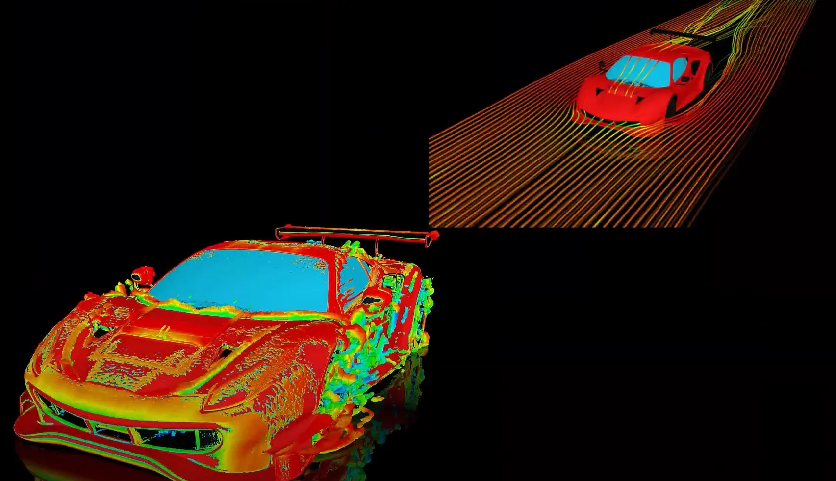
This video demonstrates exporting data from Fluent in EnSight Case Gold format, and it reviews the basic postprocessing capabilities of EnSight.
- An introduction to DO-178C
- ARINC 661: the standard behind modern cockpit display systems
- Scade One – Bridging the Gap between Model-Based Design and Traditional Programming
- SCADE and STK – Satellite Attitude Control
- Scade One – An Open Model-Based Ecosystem, Ready for MBSE
- Scade One – A Visual Coding Experience
- Introduction to Formal Verification and SCADE Suite Design Verifier
- Using the SCADE Python APIs from your favorite IDE
- Efficient Development of Safe Avionics Software with DO-178C Objectives Using SCADE Suite
- An introduction to space software standards ECSS-E-ST-40 and ECSS-Q-ST-80C
© 2026 Copyright ANSYS, Inc. All rights reserved.