Introduction

Developing an ARINC 661 Cockpit Display System (CDS) that complies with high-level performance requirements is a complex endeavor. In a previous article, we proposed a generic framework to ensure that all stakeholders work together to fit all pieces of the software inside an overall performance budget, defined by Human Factors constraints such as timely display of information and appropriate response times to air crew inputs.

The CDS server is the central piece of the cockpit; it is responsible for most of the computing workload, including drawing graphics to the various display units. Monitoring the performance of the server is therefore key to ensuring the overall performance of the cockpit.

In this article, we will take a closer look at what performance monitoring capabilities are built into the SCADE ARINC 661 server.

Note: this article assumes familiarity with the ARINC 661 standard. If you need a refresher, you may first want to read our introduction article on ARINC 661.

The SCADE ARINC 661 server

SCADE Solutions for ARINC 661 comes with tools to build a customized CDS server.

The server itself is composed of two main elements: core logic, implemented in C, and a library of widgets, developed with SCADE Suite and SCADE Display, for most of the widgets defined in the standard.

“Why deliver models & sources?”, you may ask. The reason is that the SCADE CDS server and each widget delivered in the SCADE widget library are reference implementations. Customers building their CDS will almost always tweak these implementations as they develop their server. For instance, they may wish to change the response of a ScrollList widget to scrolling: by item, by page, by pixel, with or without smoothing, etc.

In addition to sources, the product includes a build system to create the final executable. By default, it is configured for Windows host, to support development activities, but it is meant to be adapted for target builds. In the rest of this article, we’ll use the Windows host version of the server for convenience.

Overall, the CDS architecture looks like this:

SCADE CDS server architecture (left side), communicating with three User Applications (UA) and their Definition Files (DF)

Enabling monitoring

Before we start monitoring the server’s performance, we need to enable monitoring features. This is achieved by setting build option SERVER_MONITORING=ON and going through the build process.

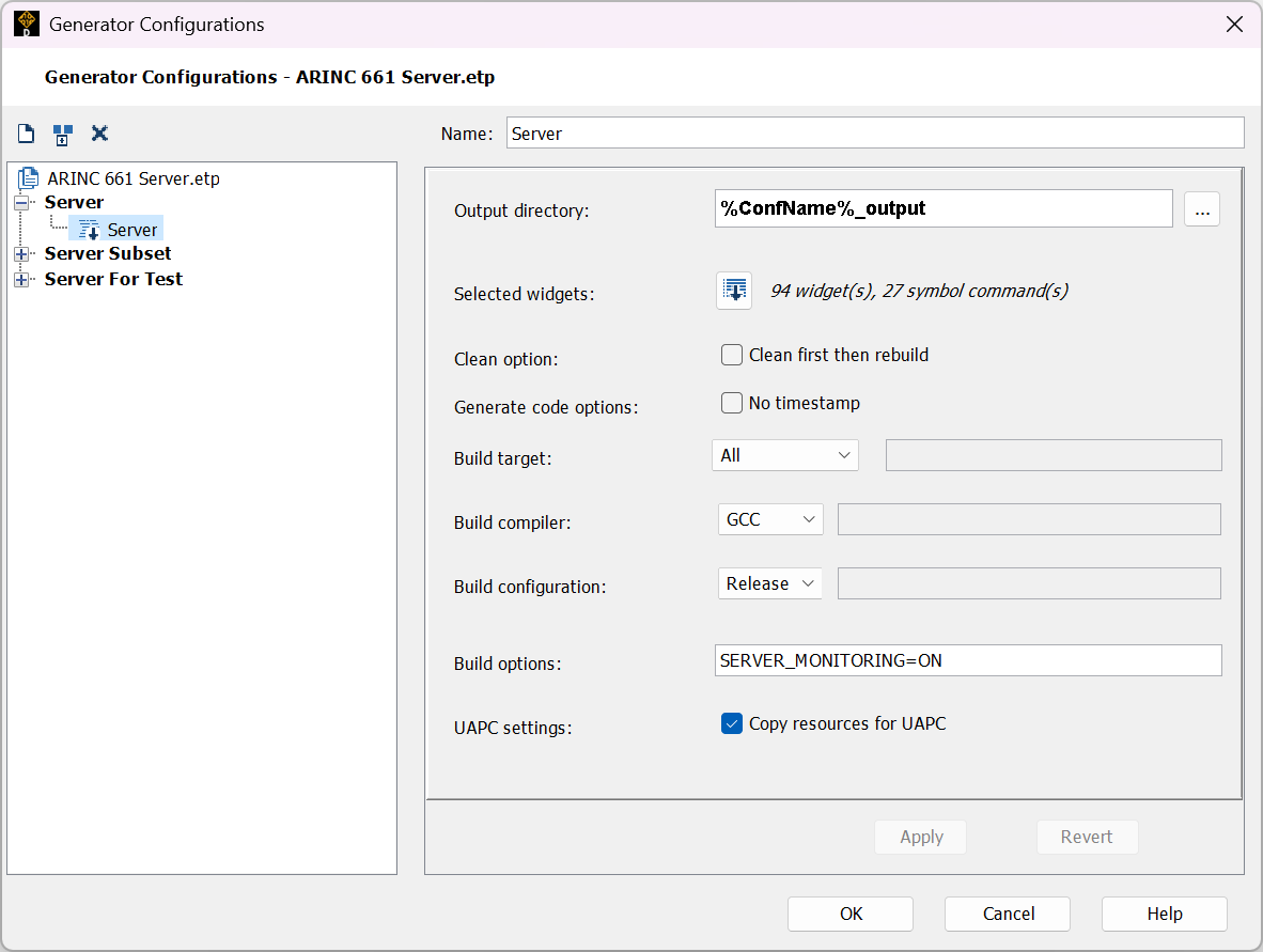
SCADE server creator with monitoring build option set

Throughout the server code, monitoring features are locked behind #ifdefs. This ensures that performance monitoring code is inactive when the server is built for production usage. This helps lighten the workload of DO-178C review activities and ensures that no computation resources are expended if monitoring is not needed.

Available options

Monitoring features in the server allow the measurement of several quantities. They can be activated either with command-line arguments when launching the server, or by pressing keyboard shortcuts at runtime.

Memory allocation (-mon_malloc), as its name suggests, captures details about RAM allocation to a CSV file. Each line lists which C source file triggered a memory allocation, which line in the source file requested it, and how many bytes were allocated.
Note that since the CDS server only allocates memory during its initial Definition Phase, the feature has no keyboard shortcut; it would make no sense to activate it during the Runtime Phase.

Execution time (-mon_profiling or CTRL+F3) prints the timing of several key tasks of the server to the console. At the end of the Definition Phase, it prints a block listing system initialization timing metrics. During the Runtime Phase, it prints key timing measurements every ~45 seconds.

Frames per second (-mon_fps or CTRL+F4) prints the frame draw time to the console every ~2 seconds.

Network payload (-mon_network or CTRL+F5) captures ARINC 661 protocol traffic to a CSV file. Each line includes the timestamp, server cycle number, direction (incoming/outgoing), size in bytes, and identifier of the remote UA. The raw bytes of the ARINC 661 message are also included.
Note: raw bytes of ARINC 661 messages can also be printed to the console by enabling server debug traces. This can be achieved by setting environment variable SERVER_DEBUG=all.

In addition to the above, option -mon_fps allows setting an output folder for the CSV reports produced by -mon_malloc and -mon_network.

Below is a cheat sheet recapping the available monitoring options:

With all this in mind, an ARINC 661 server can be launched, with all monitoring features turned on, using the following Windows batch script:

A661Server.exe ^
-mon_malloc -mon_profiling -mon_fps -mon_network ^
-mon_path %CD% ^
path\to\server_conf.xml ^
path\to\UA_1.bin ^
path\to\UA_2.bin ^
path\to\any_other_required_UAs.bin ^
path\to\color_table.bin ^
path\to\font_table.bin ^
 > a661_log_%DATE%_server.log 2>&1

This produces three files next to the launch script:

• a661_log_YYMMDD_server.log: text logs of the server, containing data from -mon_profiling and -mon_fps. Again, you may include extra debug information in this file by setting environment variable SERVER_DEBUG to all.
• a661_log_YYMMDD_HHMMSS_malloc.csv: Definition Phase report on memory allocation, containing data from -mon_malloc.
• a661_log251016_net.csv: Runtime Phase report on network exchanges, containing data from -mon_network.

The files grow in size as the server runs. If you are running this capture on your hardware target, you should ensure that enough filesystem space is available to capture them. Alternatively, if your target does not have a filesystem, you may customize the monitoring functions to log to a different output. Strategies include logging to the console, to pre-allocated structures in memory, or to a remote system via a network link.

Digging into the data

Now that we have raw data, we can analyze it. For the purposes of this article, we have run a server with several UAs that are purposefully badly optimized. During our performance capture run, the cockpit feels intermittently sluggish; let’s try to understand why.

With a couple hundred lines of Python, we can turn our raw performance logs into a dashboard:

Example dashboard, built with Python / matplotlib from the raw performance data

Uh oh – the data confirms our feeling of sluggishness. There are many things to parse on this dashboard, but we can focus on the most obvious.

First, frames per second (top left, green line) are woefully inconsistent and fall way short of our steady 50 FPS target. This is confirmed by looking at main loop time (left column, second from the top). The average (blue line) often sits above 20ms, which is the target if we are to sustain 50 FPS. Worst-case time (top of the light blue background) even reaches 140ms.

Now, why could this be? Going down one diagram (left column, third from the top), we see that Network RX (blue line) eats a large chunk of our 20ms budget. This is confirmed by looking at UA traffic (bottom right): UA 24 (purple line) is extremely chatty, with a sustained background of transmissions at every cycle and large surges of data. UA 15 (yellow green) also seems to send data each and every cycle.

These are only high-level first impressions, but we now have leads to investigate. It is likely that the two UAs above are widely overshooting their network budget and warrant a closer look. More detailed, targeted visualizations may of course be devised to identify other overshoots and refine cost functions and budgets.

Explore further

In this article, we walked through monitoring the performance of the SCADE ARINC 661 CDS server.

If you wish to play with the Python script used to create the sample dashboard above, you may download it here (or browse its sources).

If you’d like to learn more about Ansys SCADE Solutions for ARINC 661 Compliant Systems, we’d love to hear from you! Get in touch on our product page.

About the author