I tried to curve-fit viscoelastic material data, but the fit I get is very different than the experimental data I supply. I tried curvefitting with several terms, but without luck. I only read-in data for shear. I’m probably doing something wrong when curve-fitting, but I don’t know what. Could you please have a look and try to create a good curve-fit with the data I attach? The data 0.0001 100e6 .05 43e6 0.1 22e6 .15 15e6 0.2 11e6 .25 10e6
-
-
January 25, 2023 at 7:34 am
 FAQParticipant
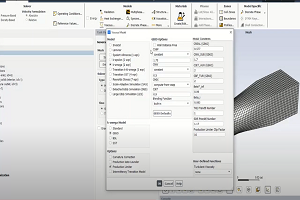
In this case, the guess that you are providing is likely sending the algorithm off in the wrong direction. ANSYS curve fitting is using the Levenberg-Marquette algorithm to perform a non linear regression on the data. One of the problems with Levenberg-Marquette is that it does not guarantee that the minimum energy condition is satisfied, that the minimum obtained using the algorithm may be a local minimum rather than the global minimum. Because of this difficulty, the judgment of the analyst is required to determine when “good enough” has been found. For the data that you supplied, visual inspection implies that Ao=1e7, A1=9e7 and tau1=.05 should give a good approximation using a 1 term Prony series. The logic here is that the Prony series will look like G = Ginfinity + G1 * exp(-time/tau1) where Ginfinity would be the value of the modulus at infinite time, G1 would be the amount of decay (in this case the difference between the modulus at zero time and the modulus at infinite time), and tau1 would be the time constant where 5 time constants represents the required time. To see this, consider the following two cases. Guess 1 assumes that the default values of 1 for all constants can be used for the curve fitting. Figure guess1a.jpg shows the setup screen from the curve fitting GUI and guess1b.jpg shows the resulting plot comparing the experimental data with the curve fit. Clearly these resultsare not acceptable. Guess 2 assumes that the initial values for the curve fit will be Ao=1e7, A1=9e7 and tau1=1, as shown in Figure guess2a.jpg. The resulting plot comparing the experimental data with the curve fit shows good agreement. The conclusion is that for non linear curve fitting, the analyst must take care to insure that the progress of the curve fitting algorithm will be in the direction of the global minimum. That poor choice for the initial guesses for the series constants will lead to poor correlations with the experimental data. Unfortunately, the ability to make good choices come from experience, and a lot of that expericence will come from making poor choices. Some suggestions can be provide. Selecting Ao as the infinite modulus will be a good choice. Selecting Ai equal to the total decay divided by the number of terms in the Prony series will be a good choice. Selecting time constants that span the entire range and that are at least a decade apart will be a good choice. Fewer terms in the series, rather than more terms in the series, is probably a good choice. One final word. The ANSYS auto time stepping algorithm does not survey the viscoelastic behavior in determining whether the time step size should be increased or decreased. At least for now, it is the analyst’s responsibility to set the incremental time step size for the problem. Experience suggests that the number of substeps should be no greater than 1/10 of the currently active Prony time constant.
-


Introducing Ansys Electronics Desktop on Ansys Cloud
The Watch & Learn video article provides an overview of cloud computing from Electronics Desktop and details the product licenses and subscriptions to ANSYS Cloud Service that are...

How to Create a Reflector for a Center High-Mounted Stop Lamp (CHMSL)
This video article demonstrates how to create a reflector for a center high-mounted stop lamp. Optical Part design in Ansys SPEOS enables the design and validation of multiple...

Introducing the GEKO Turbulence Model in Ansys Fluent
The GEKO (GEneralized K-Omega) turbulence model offers a flexible, robust, general-purpose approach to RANS turbulence modeling. Introducing 2 videos: Part 1 provides background information on the model and a...

Postprocessing on Ansys EnSight
This video demonstrates exporting data from Fluent in EnSight Case Gold format, and it reviews the basic postprocessing capabilities of EnSight.

- Question: What is the difference between PLNSOL, EPPL, EQV and PLNSOL,NL,EPEQ?
- Guidelines of modeling a gasket.
- How to use layered section to simulate composites and post process the results in ANSYS Mechanical
- ANSYS Mechanical: Delamination Analysis using Contact Debonding
- For the stress-life fatigue method, how are the Goodman and Gerber mean stress theories used to modify the calculated stress amplitude in the Workbench Fatigue Module?
- Why is the unit of the elastic foundation stiffness N/m^3?
- What are Isochronous stress-strain curves? How can they be used in ANSYS for modeling creep?
- ANSYS ACCS: Simulation of a Composite Rib Using ANSYS Composite Cure Simulation Tool
- How do I enter major Poisson’s ratio in ANSYS Mechanical?
- Hyperelastic Simulations

© 2025 Copyright ANSYS, Inc. All rights reserved.

