Exercises — Lesson 9
Exercise 1
When setting up this simulation, we chose to use the k-epsilon turbulence model. We mentioned that changing these values should not have a large impact on the results of the simulation. As an exercise, try varying the values of k and epsilon and compare them with the original results. When specifying the inlet conditions, change the method to "Turbulent Intensity-Turbulent Length Scale." Set the intensity to 0.5%, and the length scale to 0.000588m.
Enrichment Exercises
Plotting Temperature Profiles
You can look at the temperature profiles before and after the heated section.
Duplicate the Axial Velocity Profiles chart by right-clicking on the plot name in the "tree" on the upper left. Rename it "Temperature Profiles."
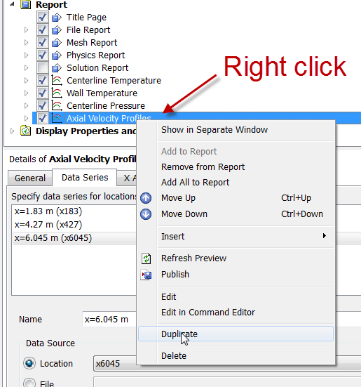
Double-click on "Temperature Profiles" in the tree view to edit its properties. This should be just below "Axial Velocity Profiles" in the list.
Change the title and x-axis variable (to Temperature). Click Apply. Here's what we get.
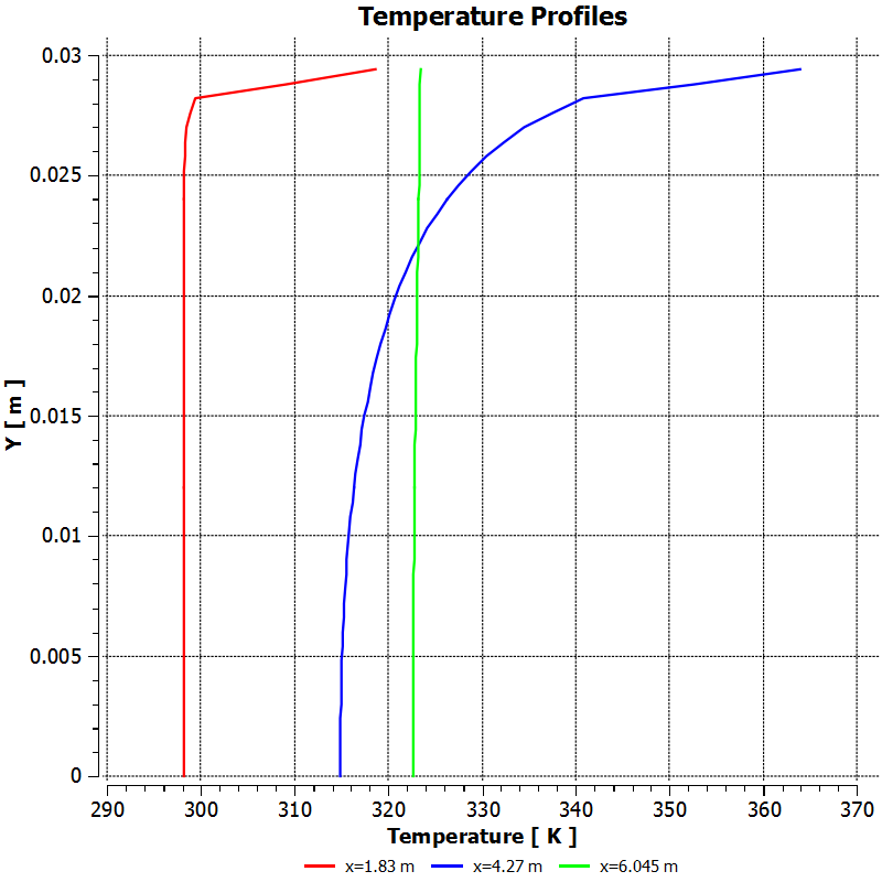
This plot shows that:
- The temperature increases in the heated section
- The temperature is much higher near the wall in the heated section
- The temperature is nearly uniform at the end of the mixing section
All these trends are as expected.
Axial Velocity Profiles
Let's look at the velocity profiles before and after the heated section. To do this, we need to first create lines at x=1.83 m ((start of heated section), x=4.27 m (end of heated section), and x=6.045 m (end of mixing section).
First, create the line at x=1.83 m.
Insert > Location > Line
Name it "x183" and click OK. Enter the following coordinates (0.0294 m is the pipe radius).
Point 1 (1.83, 0, 0)
Point 2 (1.83, 0.0294, 0)
Enter 100 for Samples. Click Apply.
Similarly create lines at x=4.27 m and x=6.045 m.
Insert > Chart
Name this chart "Axial Velocity Profiles."
Select the General tab and name the chart "Axial Velocity Profiles."
Select the Data Series tab. Change the name of the first data series to x=1.83 m. Under Data Source, specify x183 as Location.
Add a new data series by clicking on the "New" icon as shown below and repeat the above steps but for x=4.27 m.
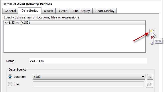
Add a third data series by clicking on the "New" icon and repeating the steps for x=6.045 m. You should then have three items in the Data Series tab.
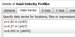
Specify x-axis variable: Velocity u
Specify y-axis variable: Y
Complete the plot. Here's what we get.
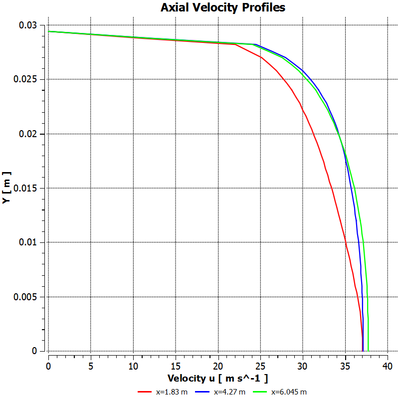
We notice that the flow accelerates due to the heating. As air is heated, its density decreases. So, the velocity has to increase to maintain the same mass flow rate.

