Ansys Assistant will be unavailable on the Learning Forum starting January 30. An upgraded version is coming soon. We apologize for any inconvenience and appreciate your patience. Stay tuned for updates.
Determine the displacements and stresses in a bike crank using 3D FEA capabilities in Discovery AIM
Verify the finite-element results from Discovery AIM by refining the mesh and also comparing with hand calculations
Problem Specification
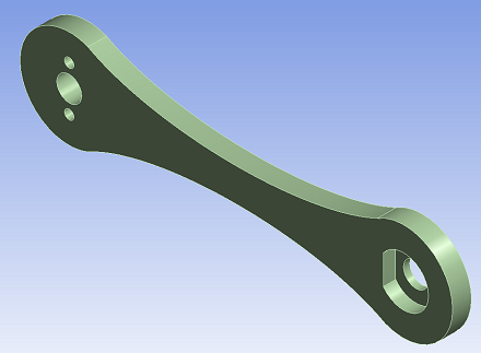
Consider the following bike crank model.
To orient ourselves, the following figure shows the location of a similar bike crank mounted on a bicycle.
Material properties: The bicycle crank’s material is Aluminum 6061-t6. The Young’s modulus is 10,000 ksi, and the Poisson’s Ratio is .33.
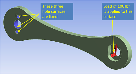
Boundary conditions: Apply a load of 100 lbf in the y-direction on the right hole surface and fix the 3 left hole surfaces as shown below. Note that this is an approximation of the actual loads and constraints on the bike crank.
The following video shows you how to navigate Discovery AIM and import the Parasolid file.
Mesh
The video below demonstrates the steps to mesh the geometry using Hexahedral elements which look like boxes. Hexahedral (or hex) elements yield higher accuracy compared with the default tetrahedral (or tet) elements for the same number of nodes.
Physics Setup
We need to create a new material and assign it to the model as shown in the following video. Otherwise, ANSYS will use the Young’s modulus and Poisson’s ratio for structural steel which is the default. This step is easy to overlook. Next, we apply the boundary conditions i.e. displacement constraints at the 3 left holes and traction on part of the right hole. Boundary surfaces where we neither apply a displacement constraint nor traction are assumed by ANSYS to be free surfaces with zero traction.
Summary of steps in above video:
Change the material from default to a newly created material
Change the properties of the new material to those of AL 6061-T6 in the problem description
Create a fixed support at the three holes
Create a force acting on the inside facing circular hole
Specify the y-component to be 100lbf
Solve the physics
Numerical Results
The following video shows how to plot the deformed shape and use it to check if the displacement constraints have been applied correctly. We next take a look at variation in stress in X-dir in the model. We interrogate variation in stress in X-dir in the interior of the model using a plane.
Summary of steps in above video:
Evaluate the 2 pre-defined results – equivalent stress and displacement magnitude
View deformation of the crank
Create a new contour to view normal stress in X direction
Create a new plane along cross-section of crank and create a new contour to view the stress variation along cross section
Create a force reaction result to check force balance
Verification and Validation
Check that the solution agrees with the mathematical model
Are the boundary conditions on displacement and traction satisfied?
Is equilibrium satisfied?
Do the reaction forces balance the applied load?
Check that the numerical error is acceptable
Are the ANSYS results reasonably independent of the mesh?
We can refine the mesh by reducing the Size Controls and updating the solution. We can then compare the results to the original mesh.
Compare with hand calculations for the bending stress and maximum displacement
Featured Articles
Introducing Ansys Electronics Desktop on Ansys Cloud
The Watch & Learn video article provides an overview of cloud computing from Electronics Desktop and details the product licenses and subscriptions to ANSYS Cloud Service that are...
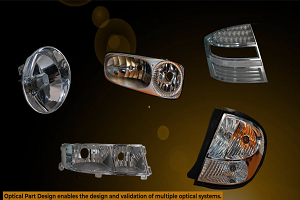
How to Create a Reflector for a Center High-Mounted Stop Lamp (CHMSL)
This video article demonstrates how to create a reflector for a center high-mounted stop lamp. Optical Part design in Ansys SPEOS enables the design and validation of multiple...
Introducing the GEKO Turbulence Model in Ansys Fluent
The GEKO (GEneralized K-Omega) turbulence model offers a flexible, robust, general-purpose approach to RANS turbulence modeling. Introducing 2 videos: Part 1 provides background information on the model and a...
Postprocessing on Ansys EnSight
This video demonstrates exporting data from Fluent in EnSight Case Gold format, and it reviews the basic postprocessing capabilities of EnSight.