Learning Forum

[m202373352]

老师您好，我在官网下载了“Inverse design of y-branch”的案例，并尝试将其修改成我自己的几何结构并进行优化，目前遇到了如下问题，烦请老师进行解答：

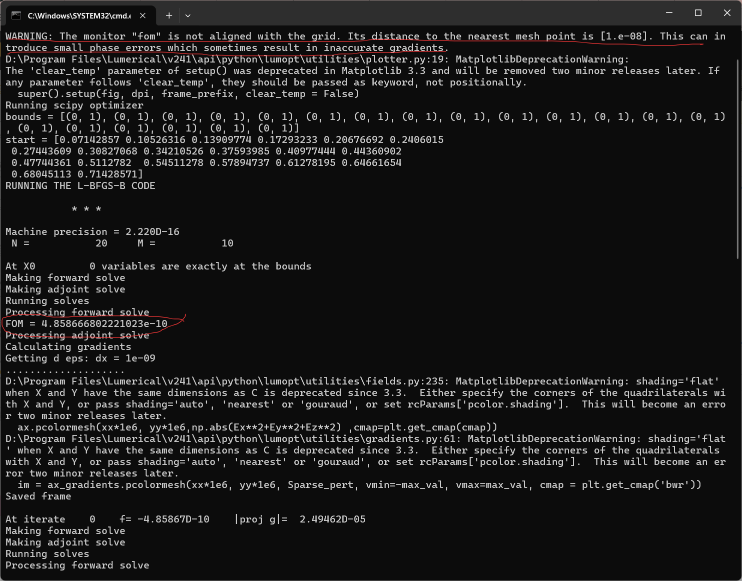
1.再将几何参数等修改为我自己的结构时，运行代码会出现如下报错：WARNING: The monitor "fom" is not aligned with the grid. Its distance to the nearest mesh point is [1.e-08]. This can introduce small phase errors which sometimes result in inaccurate gradients.但是运行案例时就没有这个问题。我也尝试在fom监视器处加一个mesh，以强制让其与网格对齐，但是这又会出现新的报错：D:\Program Files\Lumerical\v241\api\python\lumapi.py:160: UserWarning: Multiple objects named '::model::mesh'. Use of this object may give unexpected results.warnings.warn(message)。因此想请教老师，在形状优化当中，fom监视器处究竟需不需要或者说能不能加mesh以强制对齐网格？如果不能，那上述问题该如何解决？

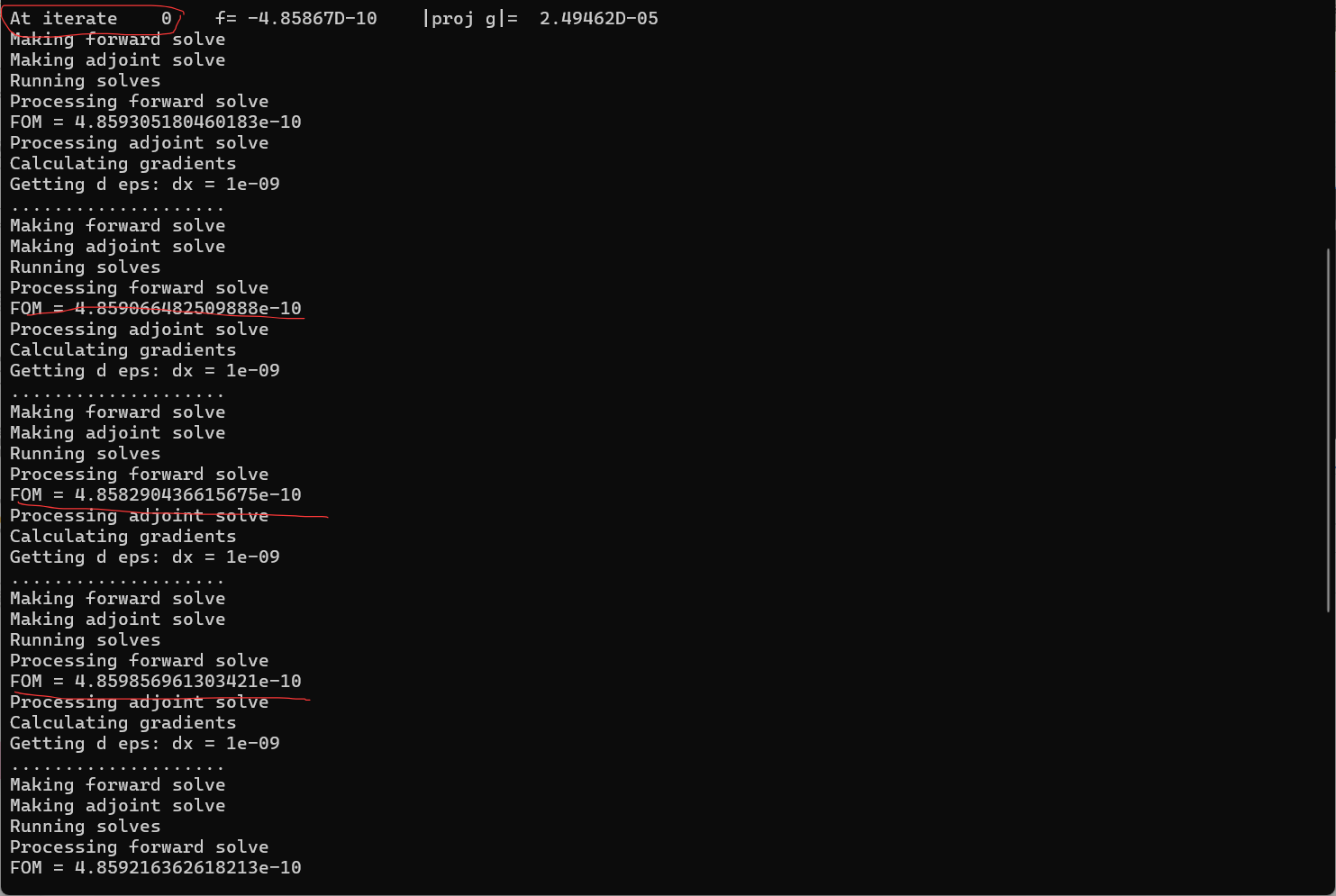
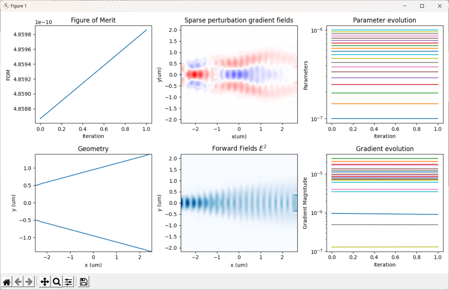
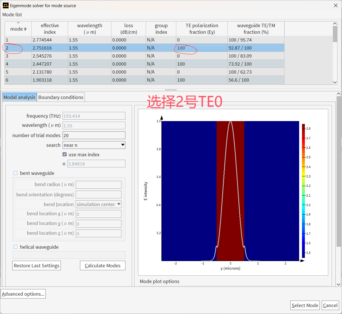
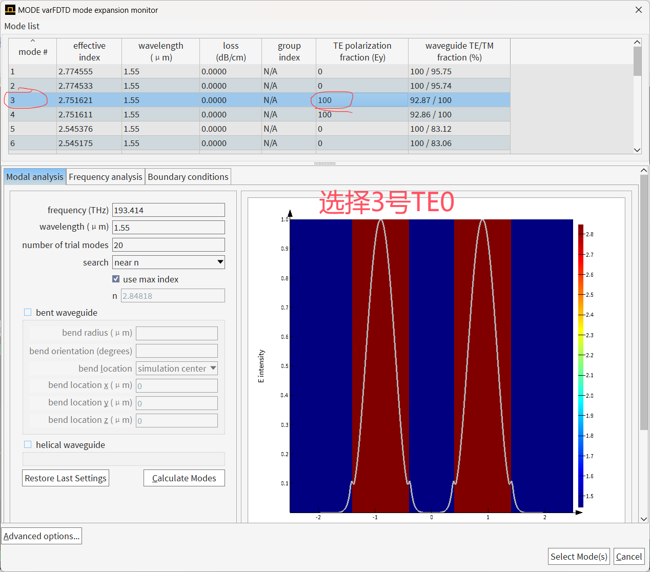
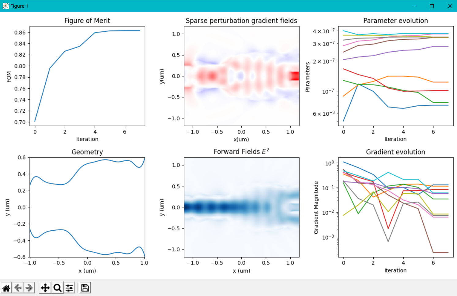
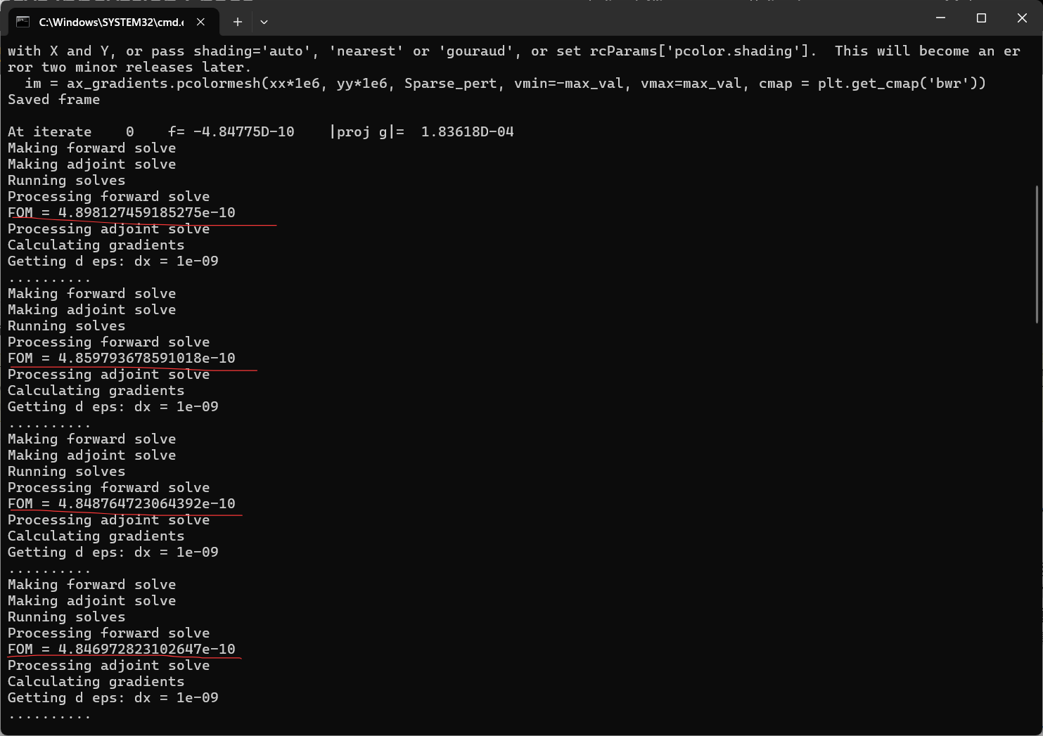
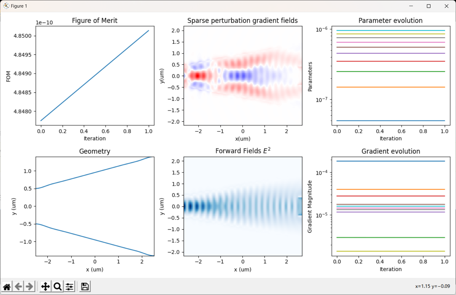
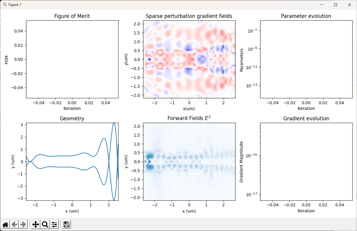
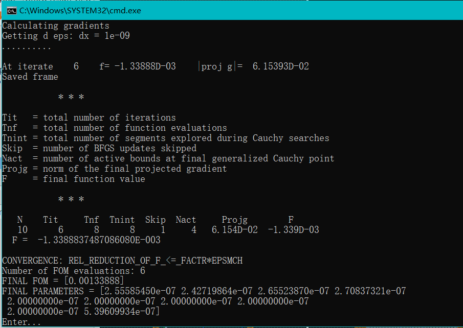
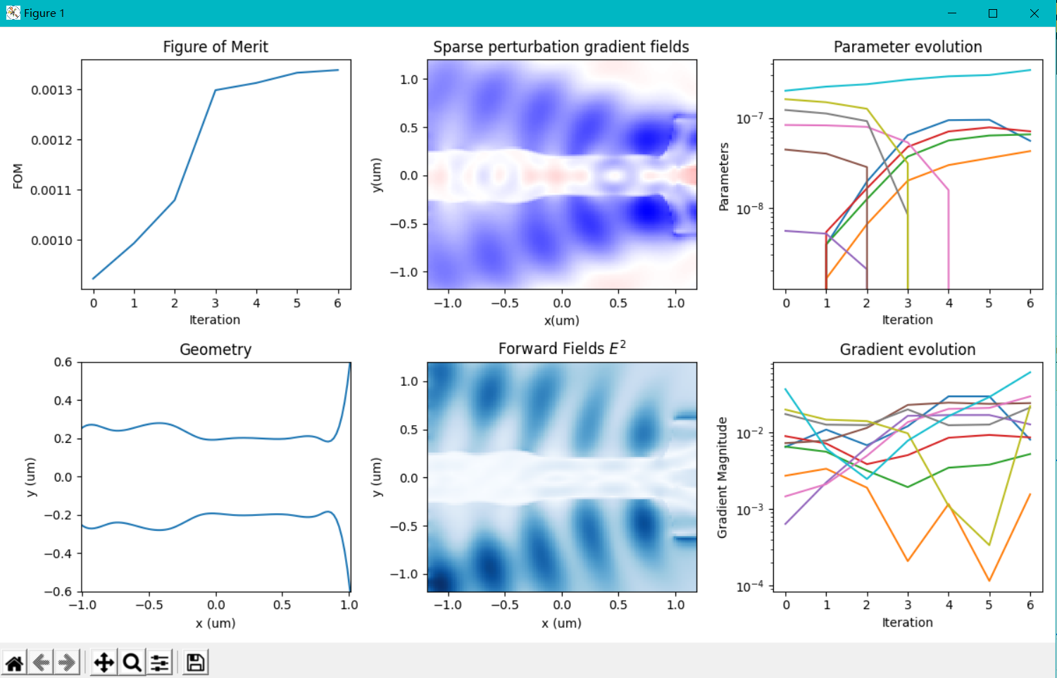
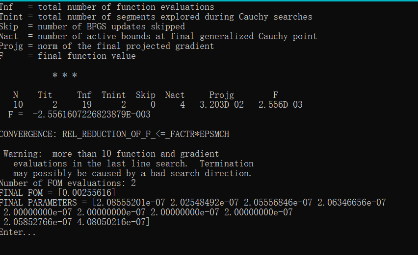
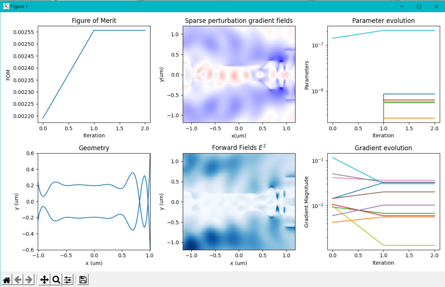
2.我在运行仿真时，并没有采用对称边界条件，因为我所选的模式光源关于y轴并不对称。举例说，我想选择TE0模作为输入，输出fom同样也选择TE0模作为监视对象，这种情况当我选择模式的序号，输入光源模式序号为2，输出fom模式序号选择3，但是发现，当直接选择模式序号时，优化会出现问题，发现迭代一直卡在第0代，并且fom值非常小（1e-10的数量级），并且几代就结束了优化，但是感觉并没有真正的优化。请问这个问题是什么原因造成的呢，应该如何解决？因为所涉及到的输入有高阶模式，因为不能直接选择“fundamental mode”。当选择输入光源和输出监视器fom均选择“fundamental mode“时，优化可以进行，但还是会出现WARNING: The monitor "fom" is not aligned with the grid. Its distance to the nearest mesh point is [1.e-08]. This can introduce small phase errors which sometimes result in inaccurate gradients.的警告。

下面给出了我仿真的代码以及相应的报错等相关截图。以上问题已经困惑了我好久，真诚希望老师能在百忙之中检阅并予以知道，非常感谢！！！！

import lumapi

import numpy as np

from scipy.constants import c

 

def y_branch_init_(mode):

 

## CLEAR SESSION

mode.switchtolayout()

mode.selectall()

mode.delete()

 

## SIM PARAMS

size_x=6e-6;

size_y=5e-6;

mesh_x=20e-9;

mesh_y=20e-9;

finer_mesh_size_x=5.5e-6;

finer_mesh_size_y=4.5e-6;

mesh_accuracy=4;

lam_c = 1.550e-6;

 

## MATERIAL

opt_material=mode.addmaterial('Dielectric');

mode.setmaterial(opt_material,'name','Si: non-dispersive');

n_opt = mode.getindex('Si (Silicon) - Palik',c/lam_c);

mode.setmaterial('Si: non-dispersive','Refractive Index',n_opt);

 

sub_material=mode.addmaterial('Dielectric');

mode.setmaterial(sub_material,'name','SiO2: non-dispersive');

n_sub = mode.getindex('SiO2 (Glass) - Palik',c/lam_c);

mode.setmaterial('SiO2: non-dispersive','Refractive Index',n_sub);

mode.setmaterial('SiO2: non-dispersive',"color", np.array([0, 0, 0, 0]));

 

## GEOMETRY

 

#INPUT WAVEGUIDE

 

mode.addrect();

mode.set('name','input wg');

mode.set('x span',3e-6);

mode.set('y span',1e-6);

mode.set('z span',220e-9);

mode.set('y',0);

mode.set('x',-4e-6);

mode.set('z',0);

mode.set('material','Si: non-dispersive');

 

#OUTPUT WAVEGUIDES

 

mode.addrect();

mode.set('name','output wg top');

mode.set('x span',3e-6);

mode.set('y span',1e-6);

mode.set('z span',220e-9);

mode.set('y',0.9e-6);

mode.set('x',4e-6);

mode.set('z',0);

mode.set('material','Si: non-dispersive');

 

mode.addrect();

mode.set('name','output wg bottom');

mode.set('x span',3e-6);

mode.set('y span',1e-6);

mode.set('z span',220e-9);

mode.set('y',-0.9e-6);

mode.set('x',4e-6);

mode.set('z',0);

mode.set('material','Si: non-dispersive');

 

mode.addrect();

mode.set('name','sub');

mode.set('x span',11e-6);

mode.set('y span',11e-6);

mode.set('z span',10e-6);

mode.set('y',0);

mode.set('x',0);

mode.set('z',0);

mode.set('material','SiO2: non-dispersive');

mode.set('override mesh order from material database',1);

mode.set('mesh order',3);

mode.set('alpha',0.8);

 

## varFDTD

mode.addvarfdtd();

mode.set('mesh accuracy',mesh_accuracy);

mode.set('x min',-size_x/2);

mode.set('x max',size_x/2);

mode.set('y min',-size_y/2);

mode.set('y max',size_y/2);

#mode.set('force symmetric y mesh',1);

#mode.set('y min bc','Anti-Symmetric');

mode.set('z',0);

 

mode.set('effective index method','variational');

mode.set('can optimize mesh algorithm for extruded structures',1);

mode.set('clamp values to physical material properties',1);

 

mode.set('x0',-2.8e-6);

mode.set('number of test points',4);

mode.set('test points',np.array([[0, 0],[2.8e-6, 1e-6], [2.8e-6, -1e-6], [2.8e-6, 0]]));

 

## SOURCE

mode.addmodesource();

mode.set('direction','Forward');

mode.set('injection axis','x-axis');

#mode.set('polarization angle',0);

mode.set('y',0);

mode.set("y span",size_y);

mode.set('x',-2.75e-6);

mode.set('center wavelength',1550e-9);

mode.set('wavelength span',0);

mode.set('mode selection','user select');

mode.set('selected mode number', 2);

 

 

## MESH IN OPTIMIZABLE REGION

mode.addmesh();

mode.set('x',0);

mode.set('x span',finer_mesh_size_x);

mode.set('y',0);

mode.set('y span',finer_mesh_size_y);

mode.set('dx',mesh_x);

mode.set('dy',mesh_y);

 

## OPTIMIZATION FIELDS MONITOR IN OPTIMIZABLE REGION

 

mode.addpower();

mode.set('name','opt_fields');

mode.set('monitor type','2D Z-normal');

mode.set('x',0);

mode.set('x span',finer_mesh_size_x - 0.1e-6);

mode.set('y',0);

mode.set('y span',finer_mesh_size_y - 0.1e-6);

mode.set('z',0);

 

## FOM FIELDS

 

mode.addpower();

mode.set('name','fom');

mode.set('monitor type','Linear Y');

mode.set('x',2.75e-6);

mode.set('y',0);

mode.set('y span',size_y);

mode.set('z',0);

 

#mode.addmesh();

#mode.set("name","fom_mesh");

#mode.set("x",2.75e-6);

#mode.set("x span",2*mesh_x);

#mode.set("y",0);

#mode.set("y span",size_y);

#mode.set("z",0);

##set("z span",240e-9);

#mode.set("override x mesh",1); ##

#mode.set("override y mesh",0); ##

#mode.set("override z mesh",0); ##

#mode.set("dx",mesh_x);

 

 

#mode.addmodeexpansion();##

#mode.set("name","mode_expansion");

#mode.set("monitor type",2); # 1 = linear X, 2 = linear Y

#mode.set("x", 2.75e-6);

#mode.set("z",0);

#mode.set("y", 0);

#mode.set("y span",size_y);

#mode.select("mode_expansion");

#mode.setexpansion("input", "fom");

#mode.set("mode selection","user select"); # use the 'user select' option

#mode.seteigensolver("use max index",1); # specify a custom value for 'n'

#mode.updatemodes(3);

 

 

if __name__ == "__main__":

mode = lumapi.MODE(hide = False)

y_branch_init_(mode)

input('Press Enter to escape...')

 

优化代码：

import os, sys

import numpy as np

import scipy as sp

import lumapi

 

from lumopt.utilities.wavelengths import Wavelengths

from lumopt.geometries.polygon import FunctionDefinedPolygon

from lumopt.utilities.materials import Material

from lumopt.figures_of_merit.modematch import ModeMatch

from lumopt.optimizers.generic_optimizers import ScipyOptimizers

from lumopt.optimization import Optimization

 

######## BASE SIMULATION ########

sys.path.append(os.path.dirname(__file__))

from varFDTD_y_branch import y_branch_init_

y_branch_base = y_branch_init_

 

 

######## DIRECTORY FOR GDS EXPORT #########

example_directory = os.getcwd()

 

######## SPECTRAL RANGE #########

wavelengths = Wavelengths(start = 1530e-9, stop = 1565e-9, points = 8)

 

######## DEFINE OPTIMIZABLE GEOMETRY ########

# The class FunctionDefinedPolygon needs a parameterized Polygon (with points ordered

# in a counter-clockwise direction). Here the geometry is defined by 10 parameters defining

# the knots of a spline, and the resulting Polygon has 200 edges, making it quite smooth.

 

# Define the span and number of points

initial_points_x = np.linspace(-2.5e-6, 2.5e-6, 20)

initial_points_y = np.linspace(0.5e-6, 1.4e-6, initial_points_x.size)

def splitter(params):

''' Defines a taper where the paramaters are the y coordinates of the nodes of a cubic spline. '''

 

## Include two set points based on the initial guess. The should attach the optimizeable geometry to the input and output

points_x = np.concatenate(([initial_points_x.min() - 0.01e-6], initial_points_x, [initial_points_x.max() + 0.01e-6]))

points_y = np.concatenate(([initial_points_y.min()], params, [initial_points_y.max()]))

 

## Up sample the polygon points for a smoother curve. Some care should be taken with interp1d object. Higher degree fit

# "cubic", and "quadratic" can vary outside of the footprint of the optimization. The parameters are bounded, but the

# interpolation points are not. This can be particularly problematic around the set points.

n_interpolation_points = 200

polygon_points_x = np.linspace(min(points_x), max(points_x), n_interpolation_points)

interpolator = sp.interpolate.interp1d(points_x, points_y, kind = 'cubic')

polygon_points_y = interpolator(polygon_points_x)

 

### Zip coordinates into a list of tuples, reflect and reorder. Need to be passed ordered in a CCW sense

polygon_points_up = [(x, y) for x, y in zip(polygon_points_x, polygon_points_y)]

polygon_points_down = [(x, -y) for x, y in zip(polygon_points_x, polygon_points_y)]

polygon_points = np.array(polygon_points_up[::-1] + polygon_points_down)

return polygon_points

 

# L-BFGS methods allows the parameters to be bound. These should enforse the optimization footprint defined in the setup

bounds = [(0.4e-6, 1.8e-6)] * initial_points_y.size

 

#Load from 2D results if availble

try:

prev_results = np.loadtxt('2D_parameters.txt')

except:

print("Couldn't find the file containing 2D optimization parameters. Starting with default parameters")

prev_results = initial_points_y

 

# Set device and cladding materials, as well as as device layer thickness

eps_in = Material(name = 'Si: non-dispersive', mesh_order = 2)

eps_out = Material(name = 'SiO2: non-dispersive', mesh_order = 3)

depth = 220.0e-9

 

# Initialize FunctionDefinedPolygon class

polygon = FunctionDefinedPolygon(func = splitter,

initial_params = prev_results,

bounds = bounds,

z = 0.0,

depth = depth,

eps_out = eps_out, eps_in = eps_in,

edge_precision = 5,

dx = 1.0e-9)

 

 

######## FIGURE OF MERIT ########

fom = ModeMatch(monitor_name = 'fom',

mode_number = 3,

direction = 'Forward',

target_T_fwd = lambda wl: np.ones(wl.size),

norm_p = 1)

 

######## OPTIMIZATION ALGORITHM ########

optimizer = ScipyOptimizers(max_iter = 30,

method = 'L-BFGS-B',

#scaling_factor = scaling_factor,

pgtol = 1.0e-5,

ftol = 1.0e-5,

#target_fom = 0.0,

scale_initial_gradient_to = 0.0)

 

######## PUT EVERYTHING TOGETHER ########

opt = Optimization(base_script = y_branch_base,

wavelengths = wavelengths,

fom = fom,

geometry = polygon,

optimizer = optimizer,

use_var_fdtd = True,

hide_fdtd_cad = False,

use_deps = True,

plot_history = True,

store_all_simulations = False)

 

 

######## RUN THE OPTIMIZATION ########

results = opt.run()

 

######## SAVE THE BEST PARAMETERS TO FILE ########

np.savetxt('../2D_parameters.txt', results[1])

 

######## EXPORT OPTIMIZED STRUCTURE TO GDS ########

gds_export_script = str("gds_filename = 'y_branch_2D.gds';" +

"top_cell = 'model';" +

"layer_def = [1, {0}, {1}];".format(-depth/2, depth/2) +

"n_circle = 64;" +

"n_ring = 64;" +

"n_custom = 64;" +

"n_wg = 64;" +

"round_to_nm = 1;" +

"grid = 1e-9;" +

"max_objects = 10000;" +

"Lumerical_GDS_auto_export;")

 

with lumapi.MODE(hide = False) as mode:

mode.cd(example_directory)

y_branch_init_(mode)

mode.addpoly(vertices = splitter(results[1]))

mode.set('x', 0.0)

mode.set('y', 0.0)

mode.set('z', 0.0)

mode.set('z span', depth)

mode.set('material','Si: non-dispersive')

mode.save("y_branch_2D_FINAL")

input('Enter...')

mode.eval(gds_export_script)

[m202373352]

以上问题已经困惑了我好久，真诚希望老师能在百忙之中检阅并予以知道，非常感谢！！！！

[GuanYo Dong]

你好

第一個指出的問題,得讓局部加的mesh name那一欄位不重複,多個編號之類的,不要讓每個都叫做mesh,這在後續select的時候容易出錯選到多個。
我們試試看比較定義座標的時候, 腳本中避免算了多次A/2,那我們讓軟件先把A/2給成一個代號每次給到軟件的位置,因為多次算可能會造成浮點數最後一個位數計算偏差,就是您看到1e-8。

第二個除了網格對不齊的問題外，我們選模式在Y-brench 出口端的兩個端口,應該各自放一個monitor去偵測,並且各自選擇模式。這三個位置的monitor也應該要一樣大,且跟結構中心對齊，此時應該選到一樣的模式編號，無論是不是自選的。

莎益博 董冠佑

[m202373352]

您的回复已经收到，非常感谢！请问"我們選模式在Y-brench 出口端的兩個端口,應該各自放一個monitor去偵測,並且各自選擇模式。這三個位置的monitor也應該要一樣大,且跟結構中心對齊"您这句话想表达的是什么意思，不是很理解？您所指的“三个位置”是哪三个位置？在Y-branch两个输出端分别放置一个监视器，还有哪个地方需要放吗？

还有就是为什么不可以像案例中那样，在输出端放置一个阔度比较大的、覆盖两个输出端口的监视器呢？

再次感谢您的回复，祝工作顺利，身体健康！

[GuanYo Dong]

你好

不好意思這個案例mode expantion的用法跟一般比較不同,他確實是兩個出口端共用一個mode expantion,並且是此結構的基模,兩個一起看總透過率。
要分析s參數的時候才一定要一個端口一個mode expantion.

另外我發現代碼varFDTD_y_branch.py,並沒有在建立基本文件的步驟加入mode expantion,但在優化文件中有 ,那你在這段落加入了,可以在優化中途確認一下是否有多一個?
如果有多,也要確認軟件抓取哪一個數據?

案例代碼y_branch_opt_2D.py就可以直接改要分析的模式,我選不是基模,可以有結果但不同的模式最佳的情況不同,這個模式就沒有官網的基模好。
所以不同模式也可能結果不好。

莎益博 董冠佑

[m202373352]

非常感谢您的回复，但是问题还是没有解决，还要跟您再请教一下。

首先，我想做一个能同时实现TE0模和TE1模分束的Y-branch结构，因而我在选择光源mode number和fom的“mode_number”时会涉及TE1模的选择，不能只选择“fundamental mode”。因为我也不知道在模式扩展监视器中应具体选择哪个模式序号，因而在fom监视器的位置放置了一个和fom监视器尺寸相同并且将fom监视器作为"Monitors for expansion"输入，用来预先确定要选择的模式序号，但是在后续开始优化的时候，我是将刚才提到的模式扩展监视器注释掉的，因而在生成的仿真文件中只有文件自动生成的“fom_mode_exp”监视器。

我在原案例代码的基础上进行了参数修改，更改了几何尺寸，即将输入、输出波导宽度改为1微米以便能激发出TE1模式，然后将中间的优化区域增大到大概5.5微米*4.5微米；并在优化python文件中，我也修改了相应的x,y坐标的范围以及bounds的范围；在选择输入模式光源的模式序号和输出fom的模式序号时，对于TE0模式，输入序号为2，输出选择3，对于TE1模式，输入选择4，输出选择8；并且边界条件为默认边界条件，没有采用对称边界条件，因为TE1模式不支持对称边界条件；其余设置均和案例中保持一致(具体代码在之前的提问中已经给出)。现在出现的问题是：当我按照上述设置进行优化时，对于TE0模式，fom的值非常小，在1e-10数量级，仿真在几代后便停止了，查看更新图像，发现参数并没有更新，意味着优化并未进行；对于TE1模式，优化在初始化完之后便停止了。具体截图如下

对于上述问题，我已经认真检查了代码，并没有发现错误，但为什么会出现这种情况就不是很明白了，还要麻烦老师予以解答，非常感谢！！

[GuanYo Dong]

你好 ,
我測了你說的情況(不設置對稱邊界,輸入輸出都挑非基模),在疊代0就數字不太好的情況下,代表沒有找到較好的優化方向,我的情況也不太好如圖
所選模式相同,不同次的結果還有些不同代表現在的結構,這可能是初值亂數選的不同了,也不是疊代越多次就一定越好,不過我沒有找到一次都沒疊代的情況。

我的理解,本就不是所有模式都找的到結構來匹配,
也看到可能一開始沒有找到好的梯度所以沒有好的結果,
這邊我感覺幫不到您了,沒有檔案能做的有限,建議您找軟件售後的AE仔細來看檔案

莎益博 董冠佑

[m202373352]

好的，还是非常感谢您的回复！