Learning Forum

[msm19b039]

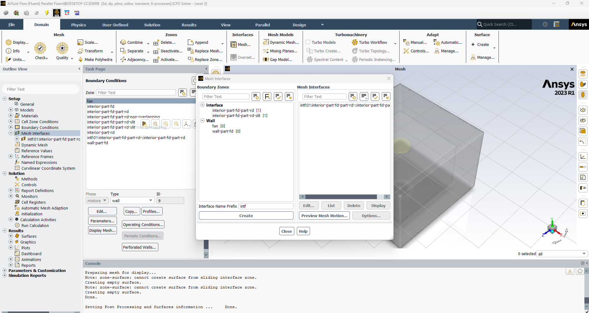
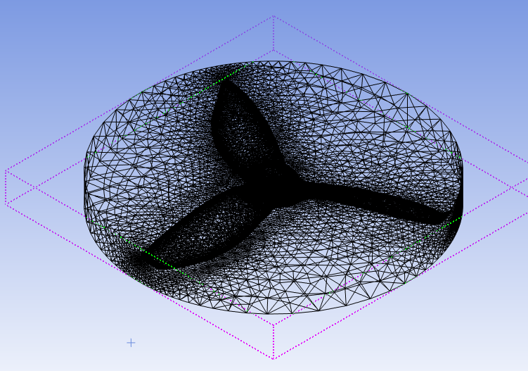
Hello everyone. I'm conducting an MRF simulation of a ceiling fan in a room. The domain(Please check image-1) is set up in a way that there is an outer chamber, inner chamber, a rotating domain(cylinder) which contains the fan. We follow this domain setup based on the directions of the Board of Indian Standards.

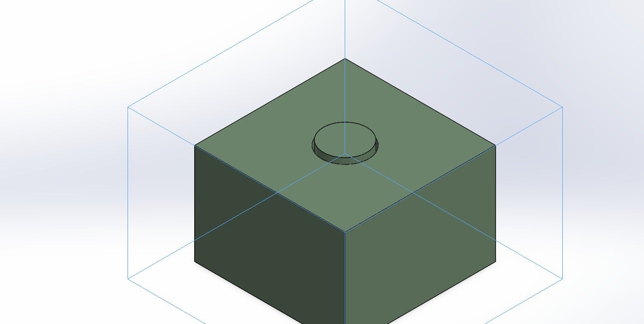
Based on widely used methodolgy, I have given 3 booleans:

1) Outer chamber subtracted from inner chamber, preserve tools 'no' and hence the inner chamber becomes walls

2) Subtract the MRF cylinder disk from the outer chamber, preserve tool bodies 'yes'.

3) Subtract the fan from the rotating disk, preserve tool bodies 'no', the fan becomes wall.

Thus I have only two bodies now, one outer chamber and one cylinder disk. I select them both and make it a single part to ensure conformal mesh interface between both.

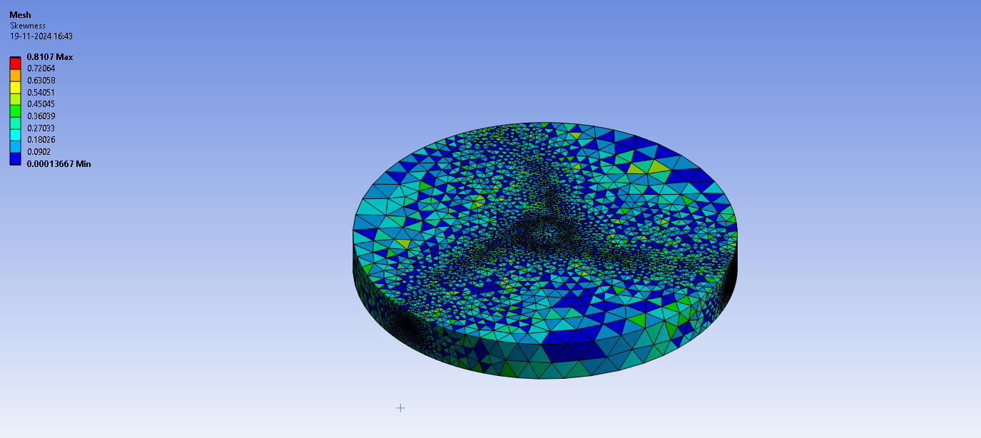
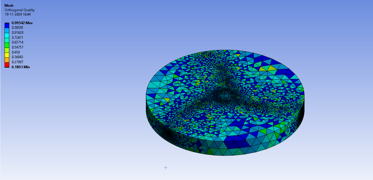
The mesh is of very fine nature with very acceptable orthogonal(>0.01) and skewness values(<0.95). I then create named selection and select the fan(hub included) faces and describe them as walls.

In setup phase, I select steady state then SA turbulence model, then cell zone is set up like this:

I've set up the coordinates of axis of rotation properly.

In boundary conditions I have set the fan to moving wall with 0 rpm. The coordinates of axis of rotation of fan are same as that of cylinder. 

I then set up the interface properly.

Then I use simple method with second order upwind.

Then I set up report definitions for fields of interest. Lift, drag, velocity average on a plane above the rotating disk and then a plane 1.5m below the disk to ensure global convergence is reached.

I then run the simulation and after my scaled residuals and variables of interest have converged. I extract the solution.

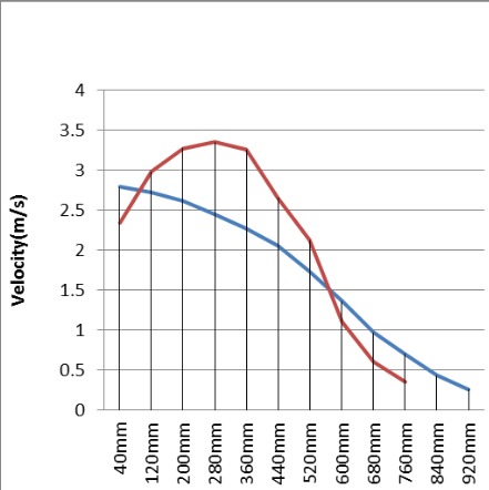
Now, If i were to plot axial velocity on a line 1.5m below the fan, from the hub to root it would appear something like the plot below(red line). The plot also shows our curve(blue line):

The red line curve is for a fan in the market. I DONT expect similar values as the operating conditions have changed. But i do expect similar behaviour i.e. like a bell curve. Every ceiling fan research paper has similar curve. Now, our new design is elliptical, has a winglet and has aifoils with changing Angles of attack over the blade but would that affect this curve? or is the simulation incorrect somewhere?

I have tried to eliminate every possible error, refined the mesh, tried the sliding mesh with non conformal, reduced time step size, simpled and coupled solver but to no avail. Im left helpless right now.

I have been investing days and nights into this since May and extreme amount of efforts have gone into this. I have a lot at stake as they want to 3D print our model for experimental investigation and I can't afford to get vague values.

Kindly help me. I'll provide you with whatever information you deem as necessary.

[Rob]

With sliding mesh I'd expect a very correct result, mrf may smooth a little based on the approach. But.... For sliding you really need the mesh to be similar size on both sides of the interface: give the tip-interface proximity that's not the case here. So, either use a lot more cells in the whole model or increase the rotating zone size by a bit (technical term). 

Another but, given the relative coarseness of the mesh around parts of the rotating zone how well resolved is the flow between the fan and 1.5m below it? Ie has any higher speed been smoothed/diffused by the mesh?

Blade profiles will have a significant effect on the flow, otherwise why wouldn't you just use a pre-bought fan? 

[msm19b039]

 

Firstly, thank you for your swift response.

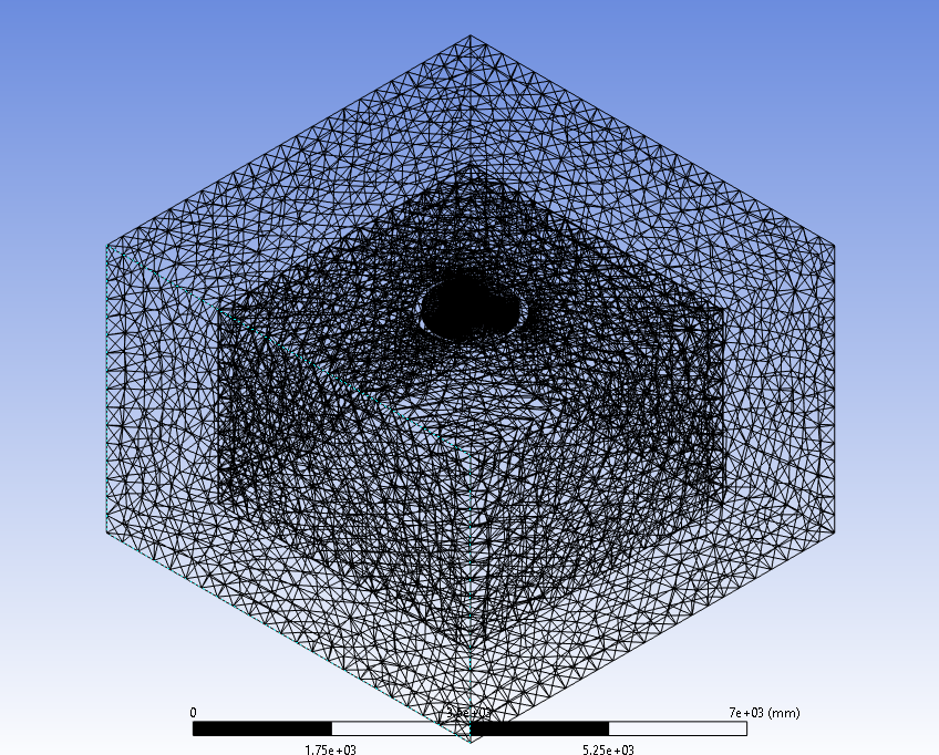
1) Say I’m using MRF, what’d you want me to do? increase the domain fine-ness by decraesing the element size? I’ve already done that. Element size currently is 280mm with 0.8 million cells. I’ve ran simulation on a mesh of 3.2 million cells as well(by giving body sizing to the rotating domain and fan and also by decreasing global element size). Neither has increasing the disk size worked.

’given the relative coarseness of the mesh around parts of the rotating zone’, as I mentioned currently I’m using a basic mesh of element size 280mm. No other additional refinements were done as a finer mesh didn’t yield positive outcomes earlier. 

’has any higher speed been smoothed/diffused by the mesh?’ How do I get to know this? I’m unaware 

 2) Blade profiles will have a significant effect on the flow, otherwise why wouldn’t you just use a pre-bought fan? Absolutely rational point but let me tell you something. I did the same study on a regular conventional ceiling fan from a literature and the plot was of the decreaaing trend instead of the bell curve which indicated that there is something wrong with the setup. 

I can attach the paper link here you can view. They do mrf and their mesh is basic with 0.7 million cells yet they get a perfect curve. Had I been able to replicate that I’d not have doubted the results of my design.

Thank you,

Expecting an early response. Grateful much.

https://ieeexplore.ieee.org/document/6778156

 

[msm19b039]

I will add a few plots here maybe they can indicate if the flow is properly resolved or not:

Velocity contour on a vertical plane midsection through the room:

Velocity streamlines on the same plane:

 

[Rob]

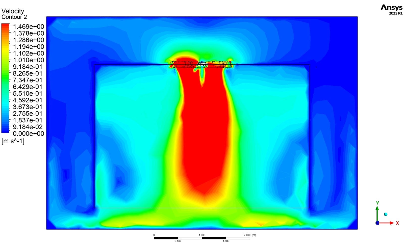
If the fan is around 1m across and your base mesh is 28cm (280mm) I'd say that was rather coarse. You can also see the effect in parts of the contour. Plot velocity in Fluent and display with node values off & focus around the fan & the reporting region. 

[msm19b039]

The length of the blade is 0.6m(sweep size is 1.2m). What domain sizing would you suggest?

[Rob]

Now look at the cell resolution at 1.5m below the blades. You're diffusing the result out too much. 

Have a look at the various examples and see what they used in the paper. Try using adaption over a cylinder starting just above the mrf, that's a bit bigger than the mrf and extends below the measuring point. Refine & run. Repeat until it stops changing. To accurately model airfoils you need to consider y+, significant levels of near wall resolution and high mesh resolution to capture the blade profile etc. In 3d that's not going to be a small model. 

As staff I'm not able to follow links and can only work with what I can see on the Forum. 

[msm19b039]

 

’You’re diffusing the result out too much’ can you please take a couple minutes to explain this? Does this mean the infomation diffusion is taking place over big sized cells instead of numerous small cells? can this be considered to be the equivalent of high courant number issue in the case of transient simulation?

’Repeat until it stops changing’ Until what stops changing? how to judge?

Your response is much awaited.

Thank you

 

[Rob]

Have a look at the training in Learning. That'll cover most of the basics, and there are a few bits on mesh resolution too. 

Re the diffusion. Consider the graph you showed above. That's made from 10-20 data points. If I were to take the curve and make a table with 3 points and then plot that would I expect to get an accurate representation of the original graph? 

[msm19b039]

 

No, I wouldn’t get an accurate representation of the plot. It will be vague. I get your point. 

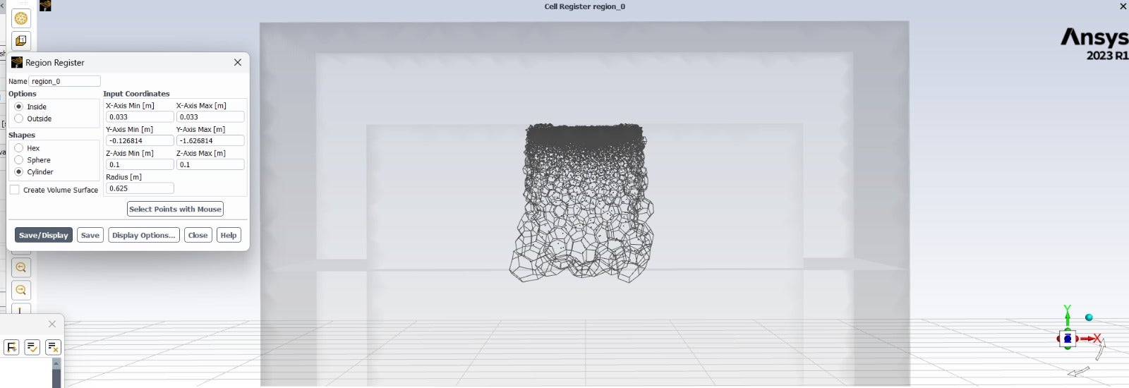
I've made the cylinder region that you suggested which captures my region of interest through cell register. I have used automatic and not manule. Please view the image below. The plane 1.5m below the fan is also shown

I'll then right click on the made register and click refine

The grid became almost 10x in size. Is this fine?

’Repeat until it stops changing’ Until what stops changing? can you just please clarify this?

 

[Rob]

You're potentially going to have a very big mesh, so for the next adaption you can bring the upper position down towards the monitor plane.  We routinely run 50-100M cells meshes so you're fine. Assuming you have the hardware. 

Until it stops changing - a mesh independence study refines the mesh until the monitors of interest no longer change. In your original model I suspect the resolution wasn't changed enough in the area of interest to make much difference. 

[msm19b039]

 

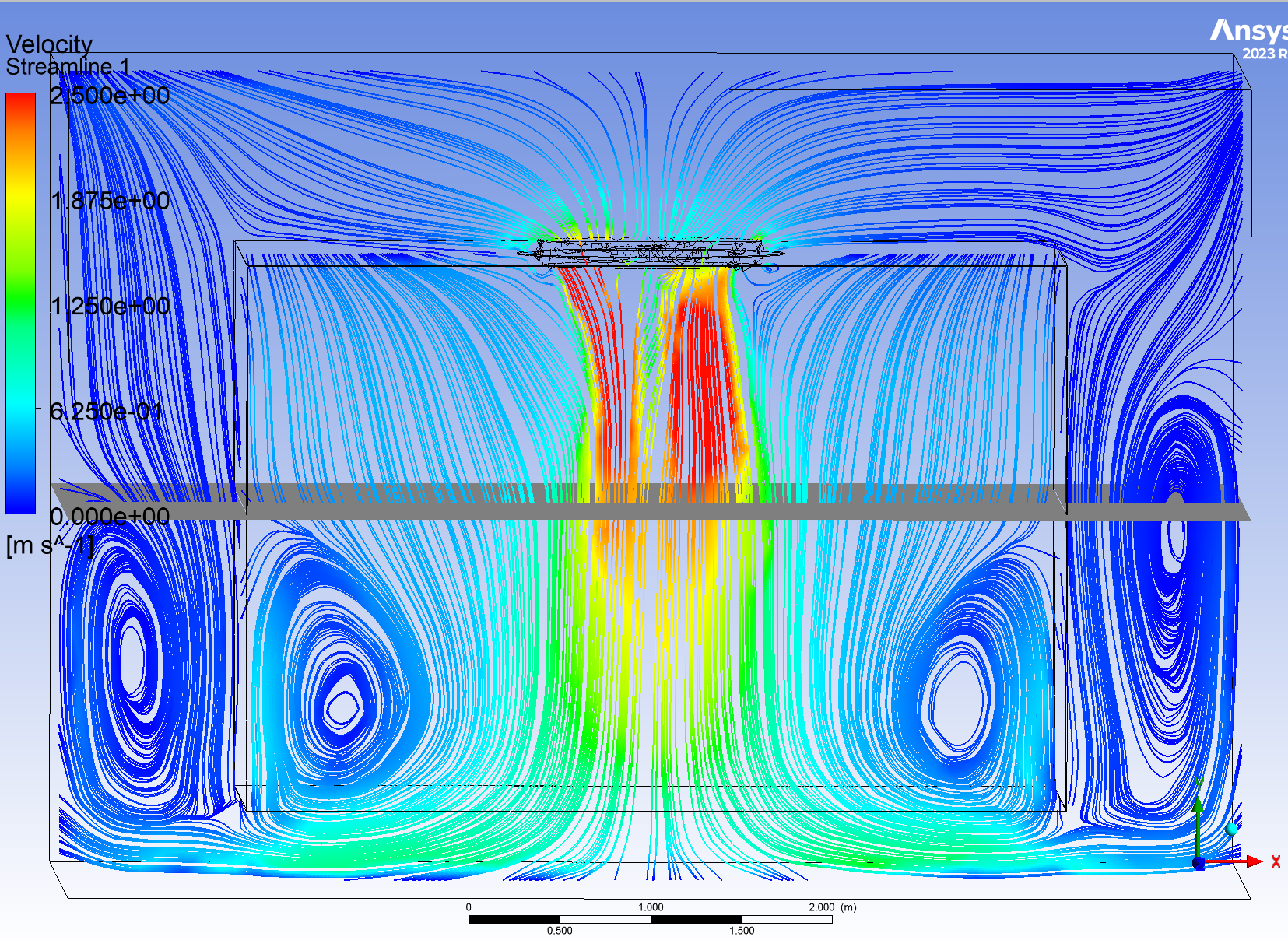
So, here is an update. I ran calculation after refining that particular cell region which increased density which I do undestand is better momentum transfer. The calculation ran only a few 1000 iterations overnight due to the size of the mesh but the initial results seem to be positive.

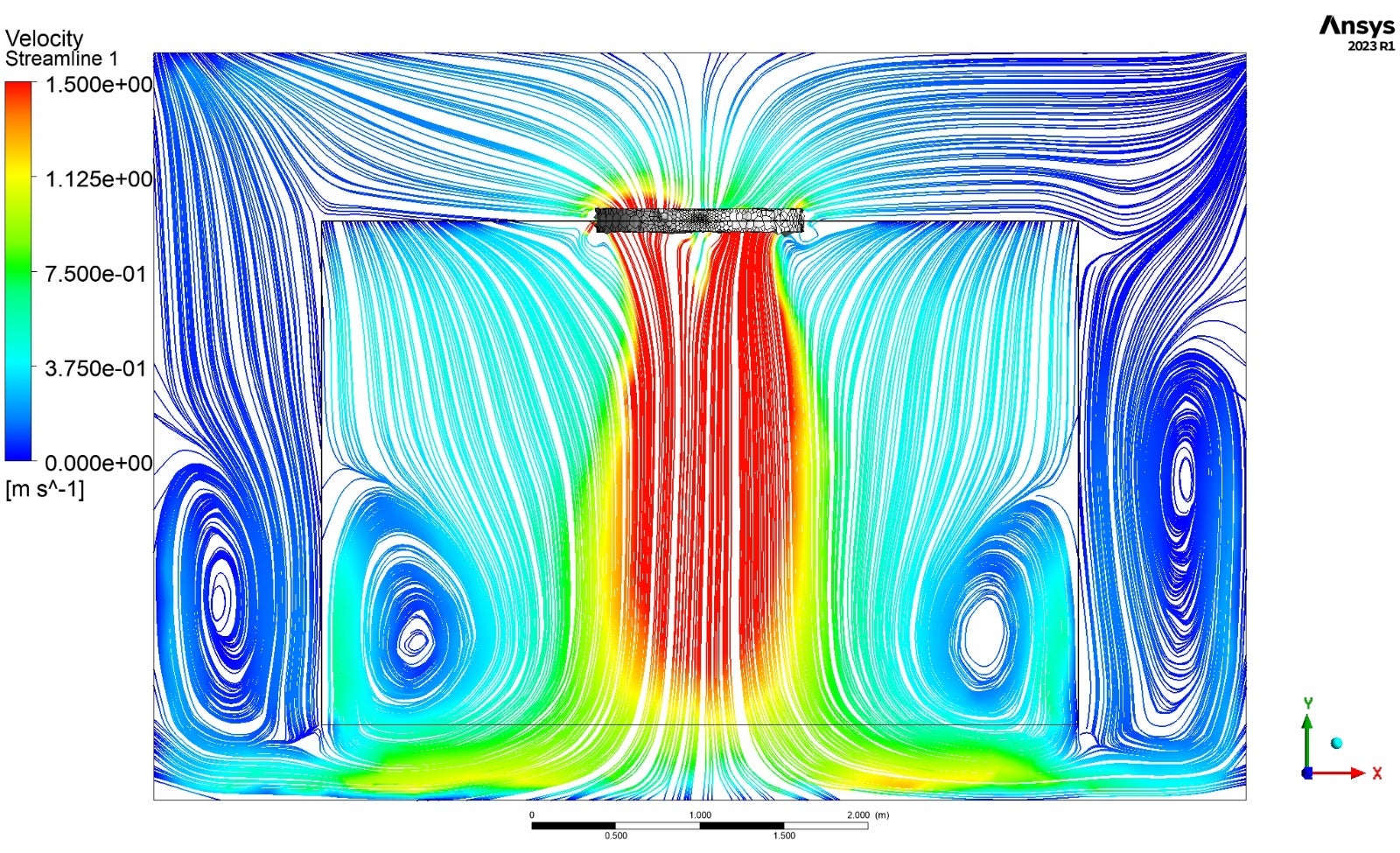
Here are velocity streamlines. I’ve displayed the plane 1.5m for better understanding. Consider a horizontal line from beneath the hub(on this 1.5m plane) to the tip, it is lesser at first then increases a bit and then decreases. Just how I said it should be.

This is how they previously were, direct decrease :

I must add this is in very preliminary stages and the simulation is running. I’ll give the next update 10-20hrs from now. 

What do you think? 

”you can bring the upper position down towards the monitor plane.  We routinely run 50-100M cells meshes so you’re fine. Assuming you have the hardware”. After creating the first cell region and refining it, I clicked on refine again out of curiosity and then fluent closed automatically with memory reallocation error which I think is regarding the cores. I’m running currently on an intel i-7 processor with 12 cores. I’m afraid this is all I can manage for now(its from my university). Also even if I make a smaller adaption region I believe it will still run out of memory. 

How is this idea though, Initially the mesh was at 280mm size, I bring it up to to say 500mm or 580mm which was default and then multiple adaptive adaptive refinement in the region of interest? This could ensure cells are placed where we need them to be placed.

The issue is that this is going to go for 3d printing in a matter of days and I can’t have my values way off the experimental ones. An error of 15-20% would still be acceptable.

Please reply. I’m grateful for your assistance.

 

[Rob]

Fans aren't that easy to model, and you may find the supply side flow patterns alter the results: I'd typically test in open space and the shroud is then dependent on the fan. Re surface mesh, once you have inflation etc you're more interested in the resolution across the blade (chord?) and then use that for the length. I don't have numbers for that, and can only point you to review literature. That high level of resolution may then need to be maintained (or at least grown slowly) into the wake region to avoid numerical diffusion. 

Core count is more for speed. RAM determines model size, coupled with poly mesh and double precision will want 3-4GB per million cells.