Learning Forum

[Sem B.]

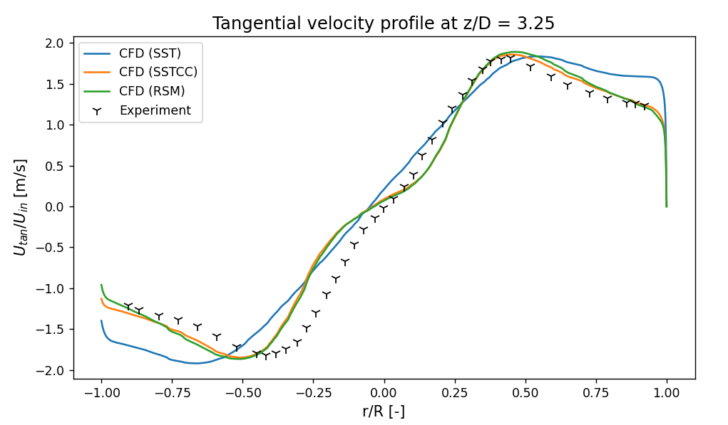
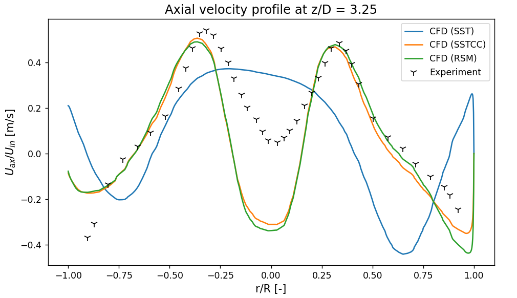
Hello, I'm trying to simulate a standard Stairmand Cyclone using the RSM model, but struggling to get it to converge and match experimental data (mainly in the center of the cyclone. I've refined to around 500.000 cells already and still the the core vortex remains to have a wide section with low tangential velocity. 

 

I've created a mesh using Fluent meshing. Polyhedral mesh with prismatic layers at the wall, using y+>30 approach (wall functions). I've extended the inlet/outlets section since this was found in literature to help get the right velocity profiles: 

 

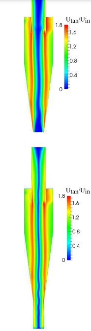
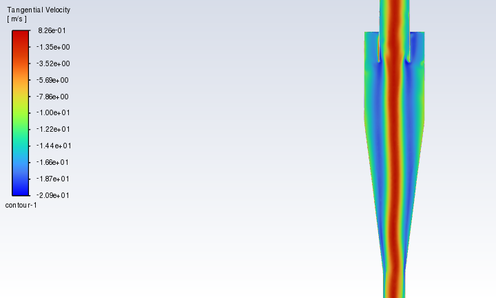
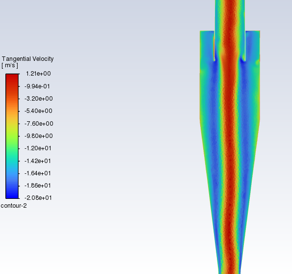
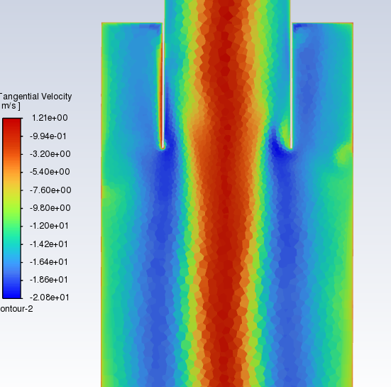
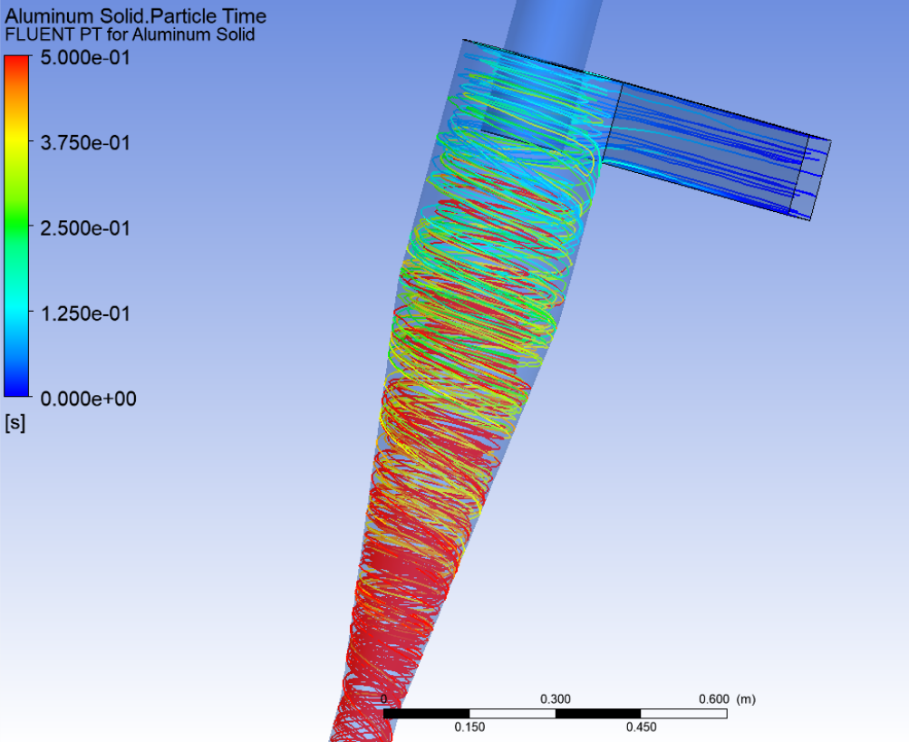
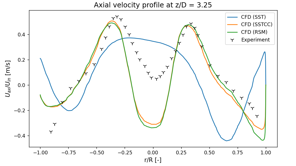
After hybrid initialization, I used SST with curvature correction to get a good initial solution before going to RSM. However, I believe SST with curvature correction should already be able to predict the velocity profiles very well, also in the core. Still, my solution keeps being like the top contour plot and the convergence remains to be rather bad. Based on literature, I don't think the refinement is the problem.

I'm using velocity inlet 10 m/s, top and bottom pressure outlet. Second order numerical schemes. Pseudo with time scale factor between 0.1 and 1.0 according to residual behavior. 

Anyone experienced with cyclone simulation that has a clue on how to solve the issue?

Thank you in advance. 

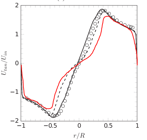
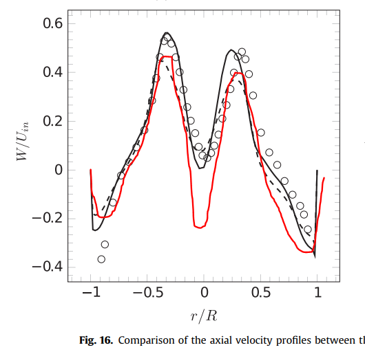
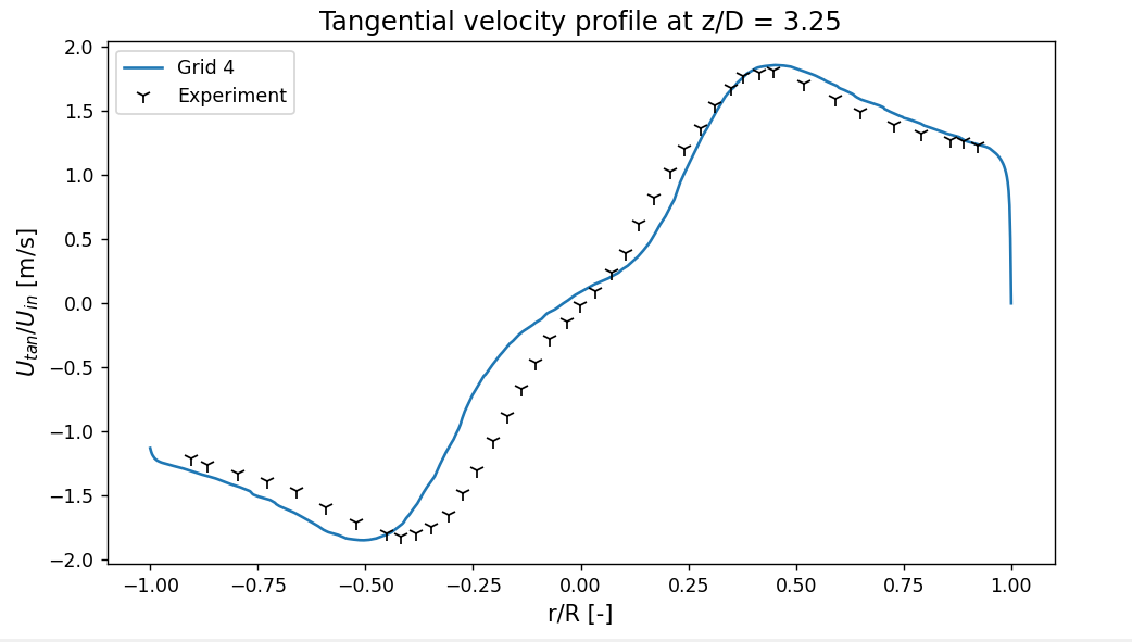
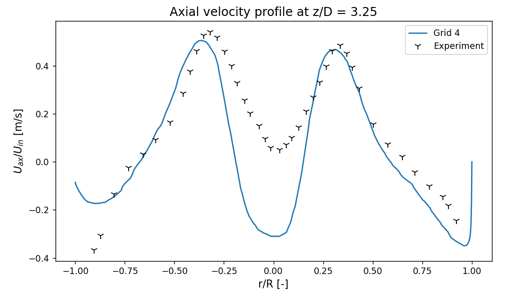
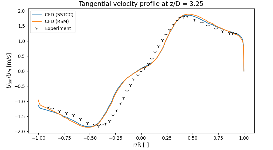
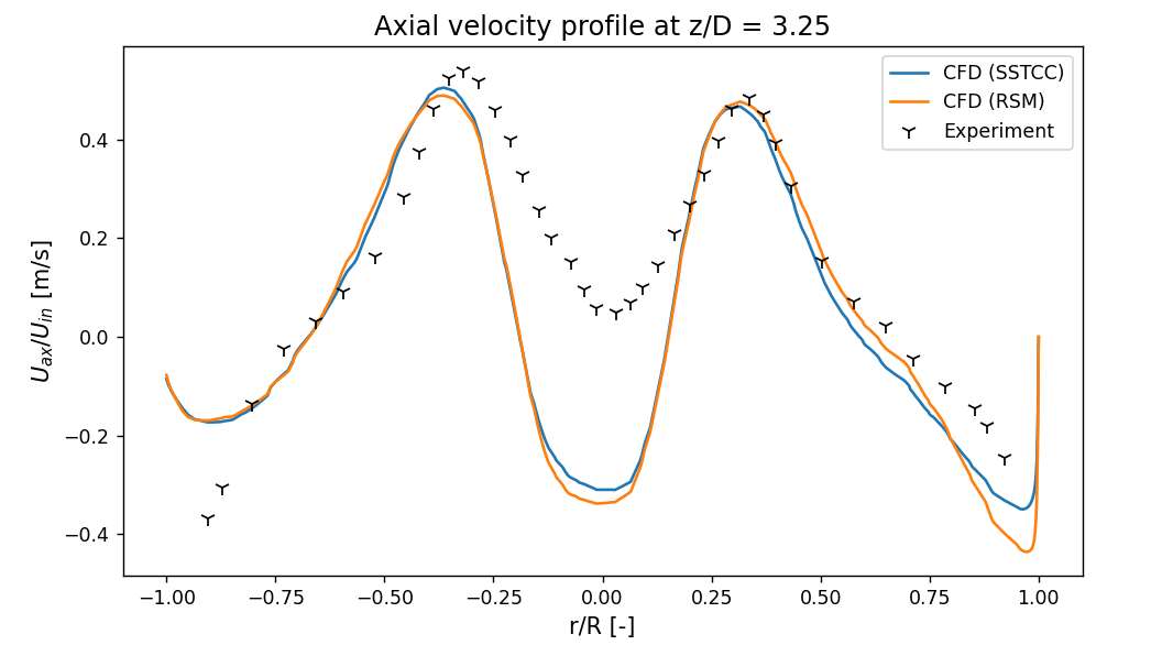
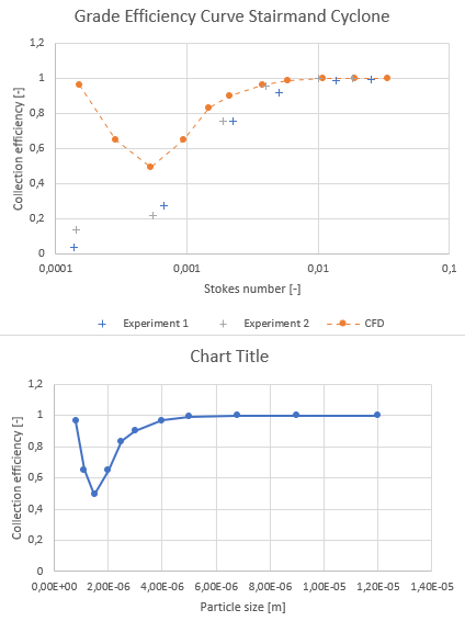
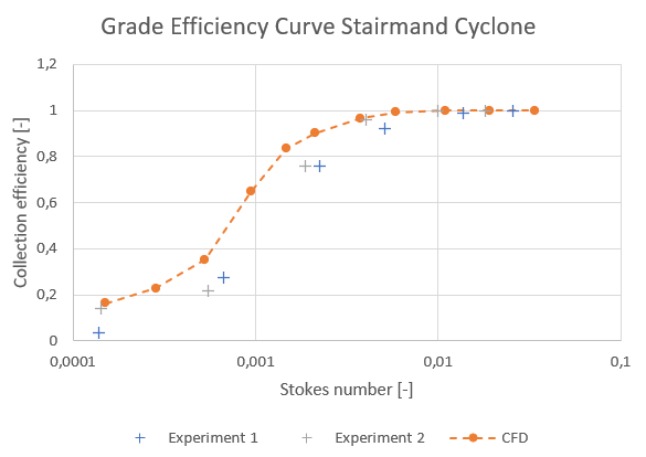
My results look roughly like this (red drawn line) w.r.t. experimental data:

[Sem B.]

Additionally, I'm getting reverse flow over both the outlets pretty soon in the simulations

[Rob]

That all sounds about right. Looking at the two contours you've nicely picked up the vortex core, and also very likely the fact that it's not fixed in place. Look at the "wobble" in the cone section. You may want to refine the mesh a little, but 500k cells should be enough: use contour plots with node values off to assess whether you're picking up the flow gradients. 

[Sem B.]

Hi Rob, thank you for your message. I'm sorry that I wasn't fully clear. The contour plots are from literature. I wanted to show that in literature it was found that extending the inlet/outlets could solve the issue of having the very wide low tangential velocity section in the center of the cyclone (as can be seen in the upper contour). However, my own results still look like the upper contour, even though I have already extended the inlet/outlets. So, for me that didn't work to get the results match experimental data. The results should look like the second contour in order to match velocity profiles from experiments.

Would you suggest me to go for transient simulation to get convergence? Besides that, what do you think about getting these reversed flow warnings (40%/30%)...

[Rob]

Plot what you're seeing. In theory you may want transient, but you also need to understand what's happening in your model. Just plotting a couple of curves isn't sufficient post processing. 

Back flow is also normal, you may want to read up on radial pressure distribution too (pressure boundary panel). 

[Sem B.]

Thank you. I'm not exactly sure what you mean, but I do have some idea. I'm also monitoring total pressure at the inlet and top outlet to see whether they are able to converge. This seems to be happening. I understand that the flow in the cyclone is implicitly unsteady. But still, the continuity residuals should be able to go at least under 1e-3, right? 

To add on the previous post, this is my contour of the tangential velocity:

 

Thank you for the tip regarding radial pressure distribution. 

 

[Rob]

Replot with node values off and then have a more careful look at the result. I can see a couple of odd features in the contour, but can't tell if it's important or not. 

A transient effect in a steady run will usually mean continuity residual hovers around 1e-2 or so. Generally the curve is fairly flat but noisy. RSM is always more difficult to converge, and generally also picks up any transient effects in the flow. 

[Sem B.]

That flat but noisy residual behavior is indeed observed. 

[Rob]

Looks OK, a bit more resolution near the core won't hurt but may not do much.  

[Sem B.]

But in that case, I'm wondering what could be a next step for me to improve the simulation results to actually match the contour (second one) I found in literature. That paper also showed that both SST with curvature correction as well as RSM should be able to predict the flow with a higher level of agreement to experimental data.

[Rob]

Look carefully at the key on the first contours. 

A colleague's written up some notes on using SST in cyclones, look in the Search function on here - I can't comment on anything that's not public and am not sure if she's had it signed off yet. 

[Sem B.]

Thank you. I found this on the forum regarding SST in cyclone simulation:

"Poly-Mesh with inflation layers at the wall.
I recommend to use either SST +Curvature Correction as start for EARSM and then RSM. In that order I will go."

Actually, that is also what I am doing: Using SST CC for intitial solution for RSM. Still, whichever mesh I use, and different settings in methods/controls, the inner section with roughly zero tangential velocity remains being much wider than expected, which can also be seen in the velocity profiles. 

I'm not sure what you mean with the key on the first contours. I have already extended the inlet/outlets by length of 2*D, which should be more than enough. 

[Rob]

The key looks to be tangential/inlet velocity? 

[Sem B.]

Yes, I noticed that it was normalized with the inlet velocity. But that is independent on the problem that I'm facing, which is the fact that my velocity profiles still look like the red lines instead of the results in literature that were produced with Fluent, which doesn't seem to change for mesh adjustments and simulation settings adjustments. I'm not sure what is causing the differences. 

[Rob]

Possibly mesh resolution? How do they compare?

[Sem B.]

 

 

Here you see the comparison of velocity profiles for different grids (grid 1 the coarsest, grid 4 the finest (505,000 cells). These results are achieved with SST including curvature correction on the polyhedral mesh with prismatic layers at the wall (y+ >30). I also noticed that some CFD-users suggest hexahedral mesh over polyhedral mesh for cyclone simulations. 

 

 

With respect to experimental data: 

 

Euler number in experiments is 5.1 [-], whereas my simulations results in roughly 20% higher value of 6.2. 

 

 

 

[Rob]

How does RSM do?  Even with the curvature correction k-w is still a two equation model so suffers from the isotropic turbulence assumption. 

[Sem B.]

Thank you again, Rob, for your help. 

These results include RSM results as well. The Euler number increased slightly to 6.3. (SSTCC: 6.2, Experiment: 5.1).

 

Ansys' guide on best practices for turbulence models explains that most of the benefits of RSM can also be achieved by enabling curvature correction in two-equation models EVMs. The results above seem to agree with this. Also, in literature I found that tangential/axial velocity profiles in cyclone simulations are often very similar between SSTCC and RSM. SST without CC produces results that clearly deviate (as expected). 

I have two ideas regarding the mismatch between experimental data and CFD results:

1) The polyhedral mesh makes it hard to capture this very narrow inner part at the center where the tangential velocity is low. A 'structured' hexahedral mesh might be a solution. However, I think that further refinement of a polyhedral mesh in that case should have also resulted in closer agreement, which is not seen in my grid convergence study (that shows that results are already (close to) grid indepedent.

2) The pseudo-transient simulations might be struggling with the vortex precession and therefore not able to capture this very narrow inner part with low tangential velocity. A transient simulation with averaged profiles over time could increase agreement to experimental data. However, would this result in closer agreement of Euler number to experimental data too? In the end, I would like to show that this approach can be used for optimization study, so transient simulations with high computational cost are not beneficial for that. 

 

 

[Rob]

I've always used RSM for cyclones, but happy to see SSTCC can give a good result. 

Mesh dependence looking purely at cell count may miss the effect of clustering cells in certain regions. I'd also check the experimental data: I'm always wary of trusting either experimental or CFD results over the other when there's not complete agreement. 

Pseudo transient may miss the core precession, so you may need transient. However, have you read any of Nick Syred's papers? They're fairly old but will be worth digging out. 

[Sem B.]

 

Thank you. Regarding the experimental data. It’s from Hoekstra (2000). I believe it’s often used in cyclone simulation. Additionally, work by Alahmadi and Nowakowski (2015) (“Modified shear stress transport model with curvature correction for the prediction of swirling flow in a cyclone separator”) showed that both SSTCC and RSM can result in better agreement to experimental data:

But as you mentioned, I might need transient for that. Regarding Nick Syred’s papers, do you have any specific recommendations regarding the point you’re aiming at? 

 

[Rob]

Nick did a lot of the earlier work on precessing vortex cores - so potentially useful for your literature review. A lot of it'll be pre-internet too. 

[Sem B.]

Thank you. I will look into it. In the mean time, I also did a transient simulation using SSTCC model on Grid 4. This didn't result in much difference. I want to evaluate the potential differences when using resolved boundary layer (y+<1) instead of wall functions (y+>30), but I'm struggling to get the mesh using Fluent Meshing. Main problem is where the tangential inlet intersects with the cyclone main body, as well as the 'bottom' of the vortex finder. Any suggestions regarding this? I've noticed that others rely on ICEM CFD or Ansys Meshing. 

P.s. for completeness of the previous plots, comparison with SST without Curvature Correction as well:

 

[Rob]

Most people adjust the geometry slightly to avoid the pinch at the inlet. Ie I chop the geometry slightly to avoid the problem. 

The vortex finder may be because inflation terminates at the end of the pipe. Not having inflation at that location resolves the issue there. 

[Sem B.]

I've done the simulation with a adjusted mesh that resolves the boundary layer (y+<1). At a first sight, this doesn't seem to make much of a difference.

Additionally, I've attempted to setup the DPM for collection efficiency evaluation w.r.t. experimental data. I've noticed that the small particles don't enter the inner vortex (and therefore escape), but they get trapped at the bottom outlet, causing an unrealistic grade efficiency curve. I don't understand why the small particles don't enter the inner vortex. 

[Rob]

Post process in Fluent. Tracks in CFD Post aren't always as reliable. How did you define the injection(s)? 

[Sem B.]

 

 

DPM:

 

 

• 150,000 steps
• Step length factor = 5
• Top outlet as escape, bottom outlet as trapped, walls reflect.

 

 

Injection:

 

 

• From inlet, uniform diameter, iterate with other diameters to get grade efficiency curve.
• Particle type: inert. 
• Drag law: spherical. 
• Turbulent dispersion: tried both none and discrete random walk (5 tries). 

[Rob]

If you've got inflation on the inlet (ie the hex cells on the inlet) you're adding more tracks from the near wall region. Try injecting from more of the middle of the inlet face: surface or similar release. 

[Sem B.]

I've tried that as well by creating a plane within the inlet tube, using the three points approach and then sample with high numbers on the two edges. But the collection efficiency for small particles remains to be unrealistically high, close to 100%. 

[Rob]

Odd as I'd generally expect the trajectory calculations to be pretty good. How does the separation efficiency curve look? 

[Sem B.]

 

These are my results with respect to experimental data: 

I must say that I came accross papers that state that the use of wall functions can result in higher collection efficiencies for small-sized particles with respect to resolving the boundary layer. However, then typically still an S-curve is seen, but then it won't go to zero for small particles, but it will go to 0.2 for example. 

 

[Sem B.]

I think I've found it. So, in the setup menu for the DPM, one can select the tracking scheme, which by default is determined through the checked checkbox 'Automated', which doesn't seem to predict the collection efficiency of small-sized particles very well in my case. Unchecking it, and selecting trapezoidal scheme seems to result in significantly better agreement to experimental data. 

Hopefully it can help others experiencing the same problem, as well. 

[Sem B.]

 

I think that now I start to understand what is going wrong with the axial velocity profiles: 

As you can see, the axial velocity is predicted too low, even negative, at the center for both SSTCC and RSM. I think this is a direct result of the backflow from the pressure-outlet at the top, that is now ‘pushing fluid’ into the boundary exactly in the same direction of the shift in axial velocity at the center. Currently, I’m using standard backflow settings, so direction normal to boundary and uniform total pressure, which is not really correct. I’m still thinking on how to improve the settings of the backflow, but I’m convinced this is contributing to the differences between CFD and experimental data. 

 

[Rob]

Try "from neighouring cell" and the radial profile on the outlet boundaries. 

[Sem B.]

From neighbouring cell has been the first adjustment I made indeed, which seems to make more sense than normal to boundary. What do you mean with radial profile? The option "Radial equilibrium pressure distribution"?

[Rob]

That's the one. 

[Sem B.]

Thank you. What about the average pressure specification option. I don't understand what it does. Is the entire backflow currently with the same pressure inserted. Does this option influence this?

[Rob]

That should be covered in the documentation, click on Help on the outlet panel.