Learning Forum

[Jason Sum]

NA

[Rob]

I suspect the problem is not the optimiser tools as such, but the fact that the two goals conflict significantly so you may need to rethink the objective function. Is the objective to minimize/maximise the flow in each direction or maximize the ratio forward-backwards? What then can be controlled to make the changes? 

[Jason Sum]

 

NA

[Rob]

I've flagged for the Optislang users as whilst I know roughly what it does, I have no idea what buttons there are to press. 

Thinking from a fluidics point of view (you may want to read up on vortex diodes, J.R. Tippetts is a good person to start with) you may want to run all of the forward and backwards scenarios and then see how the results overlay. There may be a configuration for best forward/reverse ratio but a different design maximises forward flow: goal weighting may become as critical as goal setting. 

[Jason Sum]

 

NA

[Jason Sum]

Thanks Rob. Following the previous post, grateful if Akram and Markus could offer some guides on this please.

[Rob]

Akram's looking at what he can say whilst remaining within the Forum rules for staff. 

Not sure about the adjoint bit, but I'd be surprised if you didn't have some boundary separation in the device, and that is generally unstable. Also remember that inflated meshes are just high aspect ratio cells if the flow isn't aligned (ie separation & reattachment points). 

[Jason Sum]

Thanks Rob for the updates and Akram for the followup.

Yes, I am concerning especially the tips (with inflation layers) of the tesla valve where flow diverges. Any measures or treatment you may propose in that particular regions as currently these regions are not in parallel with the flow and may cause numerical errors.(perhaps the reason leading to adjoint residual convergence issues?) 

Best Regards,
Jason

[Jason Sum]

Dear Akram, 

Was your reply removed? I am still figuring out the ways based on your guide! Thanks.

[Akram Radwan]

Hello Jason,

Let me try to reconstruct what was lost because of the database corruption. This time I have a local backup.

 

General recommendations

Do not use Ansys Workbench for shape optimization. You can prepare your calculations there. But the automation of WB can conflict with the various files the optimizer creates. I strongly recommend using the standalone version of Fluent for the optimization.

Do a sensitivity study before running the optimization. Note that Fluent can only post-process the sensitivity fields of the current calculation. To compare them, you need either separate sessions or export the results to EnSight to have both loaded at the same time. This analysis has multiple goals:

• Understand which regions of which operating condition are sensitive.
• Understand how different observable definitions might influence the result.
• Understand if or where observables support each other or are conflicting.

You can explore different optimization strategies:

• Explore different observables. Some might work better than others. For example, the velocity magnitude does not have a sign and can be maximized or minimized for the two directions. The mass flux has a sign and must be treated differently. For other boundary conditions you might need the pressure drop but measuring the total pressure drop between inlet and outlet or the pressure drop in one of the channels can lead to different results.
• You can apply a split optimization strategy. First, optimize the forward path on its own. Then optimize the reverse direction on its own. This simplifies the optimization process. Depending on the sensitivity distribution, you might want to restrict the deformability of certain regions.
• With the upcoming 2025 R1 (available in January), you can test if the optimizer can keep the mass flow rate in the forward direction above a user-defined minimum and minimize it in the other direction.

Also keep in mind that you have sharp corners in your geometry. The separation at these corners is often transient in nature, which influences the stability of the adjoint calculation more than it influences the stability of the flow calculation. The residual minimization scheme can often bring the adjoint residuals down. But you should be sure that the flow calculation is stable, i.e., stopping the flow calculation at different iterations does not show a different flow field. There are averaging methods available if this cannot be achieved but I do not recommend them before you have more experience with more stable flow calculations.

 

Boundary conditions

You have two possibilities for your BC types. You can use two pressure inlet BCs or a combination of mass flow/velocity and pressure outlet BCs.

The advantage of the pressure inlet BCs is the easy way to parameterize them. Don’t get confused by the name, when the flow goes out of the pressure inlet it behaves just like the pressure outlet BC type. You might need to initialize the flow calculation between the optimization steps, though. And two pressure BCs are not the most stable setup to begin with.

The advantage of mass flow inlet or velocity inlet and pressure outlet BCs is their stability. However, changing the BCs in an automated process is not available as a built-in method in Fluent. You need a few lines of script to do this.

But the choice of BC should be driven by what you want to model. The Tesla valve should choke the flow for the reverse direction. While it is doing this regardless of the boundary conditions, the outcome for the optimization can be very different. For pressure BCs the mass flow rate reduces, which can change the flow behavior (e.g., the existence or strength of recirculation and separation). For mass flow/velocity + pressure BCs the pressure drop changes but the general flow behavior is unlikely to change.
Consider the true operating conditions that apply to operating the device. There might be more than just the two general flow directions.

I outlined the script to change the BC-type in the other thread if you need that. Because of the limitations of scripting support especially for Scheme, I cannot provide more details. When you have difficulties, test the script line by line before using it within the optimization loop.

To initialize the flow and/or adjoint solution, search the documentation for “;@”. You can find it in the Fluent 2024 R2 User’s Guide, III. Solution mode, chapter 48.2.6. Using the Gradient-Based Optimizer, step 10: https://ansyshelp.ansys.com/public/account/secured?returnurl=/Views/Secured/corp/v242/en/flu_ug/flu_adj_usage.html%23flu_adj_sec_adjoint_grad_opt
Add a new execute command using “Execute Repeatedly every 1 Design Iteration” with the following three lines:

/solve/initialize/hyb-initialization yes
/adjoint/run/initialize
;@before-flow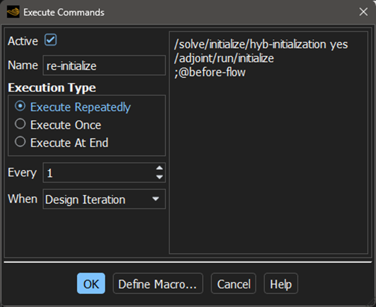

Depending on your strategy and operating conditions you might want to split this into two commands to initialize flow and adjoint separately at different steps of the optimization process.

Note: 2025 R1 will initialize automatically when you have more than one objective.

 

Adjoint convergence

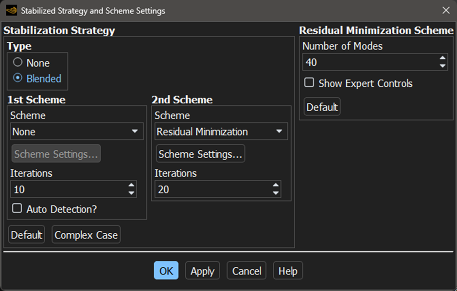
From what you have shown, I’m not concerned about the adjoint convergence. The residual minimization scheme can reduce the adjoint residuals quite reliably. If it struggles, you can increase the number of modes.
Important: Never show the expert controls of the residual minimization stabilization scheme! Just having this box checked can change the behavior of the stabilization! Only use it when you know how it influences the calculation.

Typically, I use Solution-Based Controls Initialization to reset the solver controls on initialization, 10 iterations for the first scheme without auto detection, and 20 on the second. That should be enough to converge the adjoint. If it’s not, increase the number of modes slowly. If you ever need values above 140 it’s time to think about alternative strategies and closer examination of the flow and adjoint solutions. For a better understanding, I recommend the training material for the gradient-based optimization that is available on the Ansys Learning Hub.

I also recommend taking a closer look at the flow behavior when you have convergence difficulties with adjoint. Do you have separation or recirculating flow somewhere? If yes, is this stable when you stop the calculation at different iterations or does it change slightly?
There are advanced diagnosis tools available in the text interface by keeping the cell residuals for the flow and the adjoint calculation, if you really want to dive deeper into understanding what is happening. I do not recommend this step. It requires a lot of experience to make sense out of the values that you see there. But it does exist if you want to analyze the stability on a cell level. Search the User’s Guide for “cell residuals” for the flow solver and check chapter 48.2.3.4. Printing and Postprocessing the Adjoint Equation Residuals for the adjoint solver. Again: I do not recommend this unless you have a lot of time to gain understanding of how to interpret the results with many different cases.

 

Sensitivity analysis

Taking a closer look at the shape sensitivity is often ignored but it can give you valuable insights. The quantities you want to look at are the log10 shape sensitivity or the surface shape sensitivity. The first one is a logarithmic scale of the shape sensitivity, which makes it easier to see the distribution because it has a very large range. The second one is a smoothed version of the shape sensitivity.

I recommend to start with the surface shape sensitivity but before you do, change the postprocess options that you can access from the Design ribbon. Make sure the surface shape sensitivity is set to spring. The default radial basis function approach can be computationally expensive. Whichever method you use, this is just to get an impression of the sensitivity distribution, it is not used for anything by the mesh morphing. The Design Tool uses the raw shape sensitivity and applies the smoothing during the morphing process, which depends on the selected morphing method.
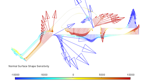
Unfortunately, it is not possible to export the surface shape sensitivity vector components to EnSight. If you want to use EnSight for a direct comparison, use the unsmoothed shape sensitivity components instead.

Use vector plots for 2D cases. For 3D cases it is often more convenient to start with contour plots of the normal surface shape sensitivity. Check the regions of high absolute values for both flow directions.

• Are the regions similar?
  • If yes, is the sign identical (general direction of the vector)?
    • If yes, both observables support each other, it’s just a question of scaling them appropriately.
    • If no, either the observables are in conflict with each other. Optimization without defining trade-offs is either very challenging or even impossible.
  • If no, how different are they? Would it be possible to concentrate the shape change of one flow direction to certain regions and the reversed direction to different ones?
• How different are the absolute values of the shape sensitivities?
  • Remember that the shape sensitivity has a unit that depends on the selected observable. If the observables are comparable (e.g., both use the average velocity magnitude at one boundary), differences indicate how to scale the objectives.

Based in the outcome of looking at the shape sensitivities you can derive an optimization strategy.

Remember: depending on maximizing or minimizing the observable, you might need to reverse the direction of the sensitivity vectors!

 

Optimization strategy

As indicated initially, there are different strategies possible. The flexibility of the optimizer is limited in favor of a fully automated workflow. Depending on the strategy that you want to use, you might need to do this manually.

Standard approach
Based on the sensitivity analysis, you can set you objectives and hope for the best. While this works well for a single objective, it rarely works for multiple objectives or conditions.

Consecutive optimizations
This approach works best when the sensitivities have their extreme values in different regions of the domain. It is mostly useless when they are in conflict everywhere. Just run the optimizations with a single objective/condition. Once this cannot be continued, change the flow direction and run a new optimization.
You can also change the region easily with this approach, for example, to optimize the straight part of the pipe for the forward calculation and the bended part for the reversed direction.

Customized approaches
Obviously, there are more approaches.

Similar to the consecutive approach from above, you could do this in one step. There is no tool in Fluent to automate this apart from writing your own full optimization script. The idea is to set the first condition, calculate flow and adjoint, set the region and design conditions as needed, and morph the mesh. Then switch to the second condition and repeat. With this alternating approach you can run a combined optimization but with different settings for the mesh morphing.

You can also use different observables for the directions. I didn’t test this. But you could come up with an idea to maximize the flow rate through different parts of the domain, e.g., for the reverse direction maximize the flow rate through the bend, for the forward direction maximize the flow rate through the outlet. You can implement this in the optimizer by setting an objective to ‘none’ for the condition where it is not relevant. This will still calculate the adjoint for it, but it is not considered during mesh morphing.

As indicated above, 2025 R1 offers new methods for the optimization that can be useful for a case like this. You can implement a similar procedure yourself. Just run a single-objective optimization but stop it when the observable for the other operating condition is outside the bounds (e.g., the mass flow rate for the primary flow direction drops below a user-defined minimum). Only if this is the case, optimize for the other direction until it is well above the threshold. Then continue with the first set of settings.

There are more. I hope you get the idea that there is not just the workflow that is implemented in the gradient-based optimizer. That is the most common one, but not the only one. Understand the sensitivities. Then derive a workflow to change the shape in a promising way.

 

Conclusions

Optimizing a Tesla valve design is not the most trivial task.

1. Start with the boundary conditions. Which ones are reasonable to describe the physics of the problem?
2. Shed a thought or two about local stability of the flow calculation.
3. Think of possible observables. There are often more than one possible objective functions and because of the nature of the adjoint method the resulting shape can be quite different.
4. Analyze the sensitivities for the different operating conditions and observables. Understand where they support each other and where they are in conflict.
5. Derive possible optimization strategies. Not all of them are available as built-in capabilities. Be creative, then simplify.
6. Run the optimization. Analyze how it performs. Fine-tune the approach or use one of the other strategies.

I hope I didn’t miss a question and that I covered all of the lost information.

[Jason Sum]

NA

[Akram Radwan]

1) Workbench and shape opt

The recommendation against Workbench is strictly for the shape optimization in Fluent. The gradient-based optimizer writes multiple files that Workbench does not really know what to do with them. Furthermore, even the manual process deforms the boundaries, which invalidates upstream connections. Therefore, I recommend using the standalone version of Fluent for the shape opt process to not delete optimization data by accident.

For parametric design changes, Workbench is a good tool also in combination with Fluent.

2) Sensitivity analysis

After you run an adjoint calculation you have additional field variables available. You can process them in Fluent or in dedicated post-processing tools like EnSight.

3) Convergence

Convergence is a challenging topic especially in the context of adjoint calculations. It is too broad to discuss all the details in the forum. I could easily deliver a two-hour lecture about this topic and still not cover everything. If the flow doesn't converge, you should expect serious convergence difficulties with adjoint. If the residual minimization scheme can bring the residuals down, you are not necessarily 'safe' in terms of accuracy. You might have local instabilities in the flow calculation that give you a stable adjoint result, but the sensitivities could depend on the point when you stop the flow calculation. Check the behavior close to sharp corners and separation in general to get a better idea about the impact on the optimization.

4) 2025 R1

The version is available in the download portal already for early adopters. The official announcement should follow soon.

[Jason Sum]

 

NA

[Akram Radwan]

I'm not aware of an official way to get the scaled residual values. You can keep the cell residuals with the TUI "/solve/set/advanced/retain-cell-residuals y". They are unscaled. Therefore, I'm not sure how useful they are for your purpose.

There is an RP var to indicate convergence: "solution/converged?". It's just true or false based on the last calculation of the case. When just reading the cas file, it is the status the last time this cas was saved, regardless of the available data at that point in time.

I don't know if the Fluent node in optiSLang evaluates this status automatically. If not, you would need an output parameter for it by setting the RP var into an output parameter for DX and optiSLang. You can probably do this with an Execute Command. Note that there are defects in several versions of Fluent that prevent under different circumstances the correct execution of commands that include the \", which is needed here to use quotes inside a string. As far as I know, it should work in 2025 R1. But I haven't tested it. If it doesn't work correctly, you can move this line into a journal and load the journal from the Execute Command. The line expects an existing expression with the name "convergence_status".
(ti-menu-load-string (format #f "/define/named-expressions/edit convergence_status definition \"~a\" q" (if (%rpgetvar 'solution/converged?) 1 0)))

[Jason Sum]

 

NA

[Akram Radwan]

As Ansys employees, we cannot debug UDFs. Maybe you can open a separate thread for this if the error persists to get help from other users.
Reading and understanding error messages is critical to find UDF errors.

udf_names.c(6): error C2449: found '{' at file scope (missing function header?)
Your code has an incomplete #include statement at the top.

udf_names.c(18): fatal error C1004: unexpected end-of-file found
You probably have an incorrect compiler directive (see #include) or there are unclosed braces.

In general, when you face compiler errors, you can always strip down the UDF to the bare minimum, e.g.
#include "udf.h"
DEFINE_ON_DEMAND(dummy)
{Message("finished.\n")}

Then copy your intended code line by line / block by block into this to see when the compiler error appears to locate the source.

[Jason Sum]

 

 

 

NA

[Jason Sum]

 

Dear Akram, 

I would be grateful if you could guide me further when you are available, please and appreciate!

 

[Akram Radwan]

Dear Jason,

It's a good idea to start with one direction and make the problem more complicated in a second step.

 

Workflow

The workflow is correct. There are cases where the automatic convergence detection of Fluent stops the flow calculation at the first iteration after mesh morphing. Typically, this is the case for cases with very small changes to the surface mesh. You can either disable the convergence check completely unter Monitors > Residuals or set the reporting interval on the Run Calculation task page to a larger number than 1. The second method only works if there is a significant jump of the residuals in the second or third flow iteration.

 

Adjoint Residual

As long as there is progress towards convergence, you can ignore the warning messages about the preconditioning. Usually, this means that the automatic adjustment of the Courant number for the adjoint solver is a bit too aggressive. But if the residuals drop reliably, you can disregard the messages.

 

Observable Target

It can work to start with larger steps but it does not have to. Usually, we recommend using a small step size for a single step. The adjoint method assumes linear behavior and flow residuals of zero. Flow problems are always non-linear and our residuals are never zero. So, there is a certain uncertainty associated with the sensitivities. By going in small steps, these uncertainties are small and the sensitivities guide the shape towards the optimum.
However, this will give you only one local optimal solution, based on the initial geometry and flow behavior. When you use a very large change for the first step, you might jump over this initial local optimimum and find a completely different solution. This could be better, worse, or identical to the optimal performance when using small steps.

 

Mesh quality

The optimizer tries to improve the mesh quality three times after the mesh morphing by default. Essentially, this is just the text command /mesh/repair-improve/improve-quality. There are limitations to what this method can do. And for larger surface mesh changes you also might end up with very large cells in certain regions which leads to under-resolving local gradients. The only solution to this is a remeshing step, preferably in the original mesh generator. Note that an STL export is only possible with 3D cases.
The quality criterion in the optimizer has a different effect. When the mesh quality before the improvement step is below the specified criterion, Fluent reduces the step size (target change) automatically because smaller mesh changes have a lower probability of reducing the mesh quality significantly.

[Jason Sum]

NA

[Jason Sum]

Dear Akram,

Sorry to bother, I will be so grateful if you could give me further directions. Currently the morphing is so insignificant no matter using outlet flowrate or volume interal turbulence as observable (sensitivity not high enough?). I do not know any attemps or settings that would guide me to a way towards significant morphing for optimisation. Huge thanks.

[Akram Radwan]

It is difficult to analyze the behavior without having access to the case. Obviously, this would require a commercial support contract. We're very close to the limits of what we can support through the forum already.

I created my own case to have something to play with. Dimensions and BCs are different from your case. Therefore, I do not expect identical behavior. Still, I would have expected a somewhat similar sensitivity distribution, which does not seem to be the case.

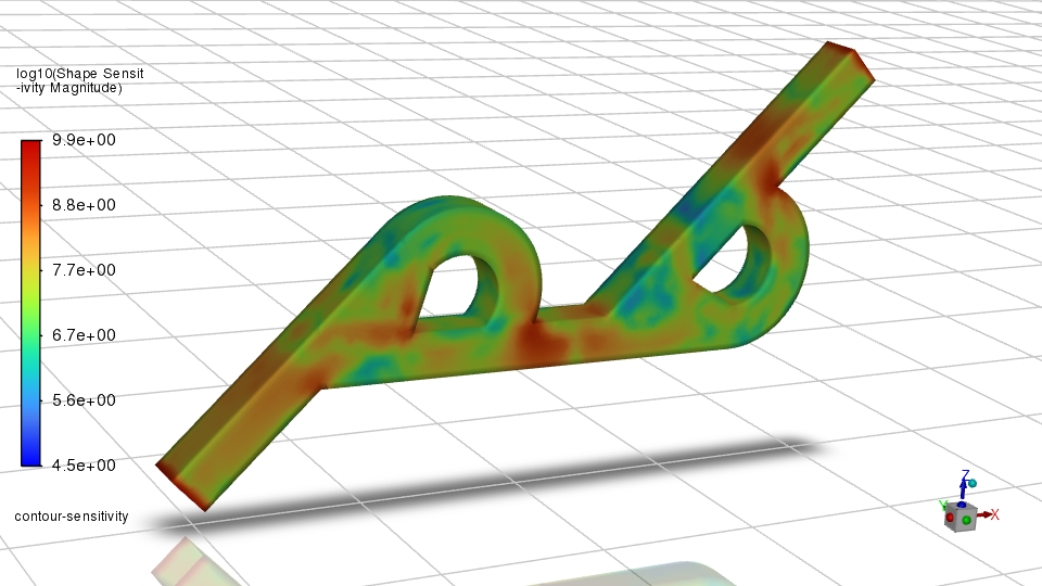
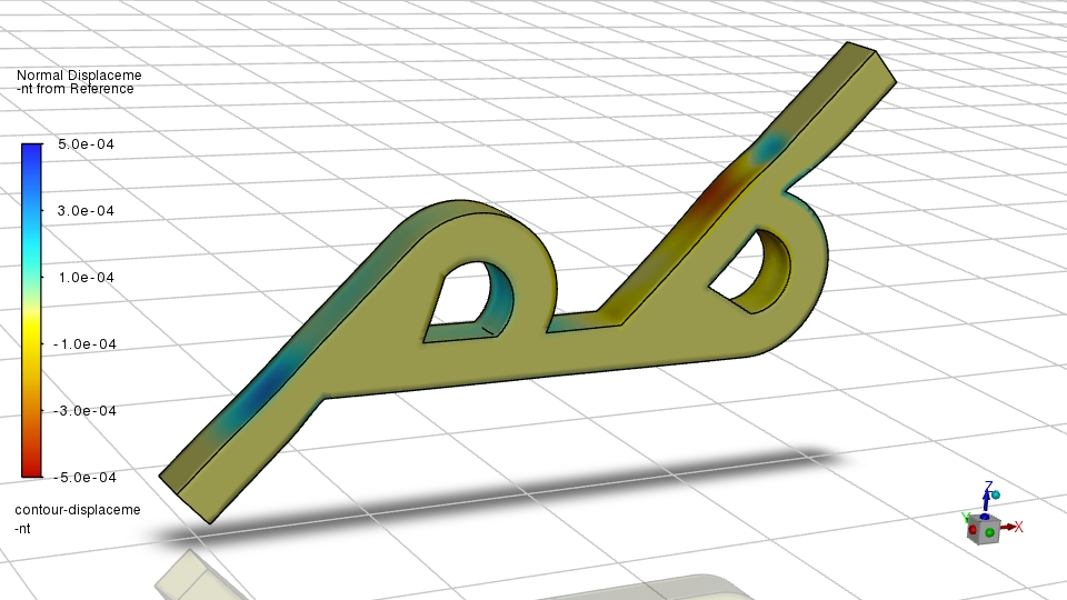
I can only guess that there are some inherent differences in the flow behavior between your and my case. Especially the very asymmetric blue spots at the second pass are unexpected, at least if the plot is from the initial geometry.

The next question is which deformation would you expect? The goal is the reduction of the mass flow rate. The easiest way to achieve this is to choke off the flow by moving the region at the first corner inwards. This is also shown with the sensitivity plot.
There are two noteworthy observations for this:
1. Your sensitivity plot has a very clear highlight only at this corner. This is not so clear with my case where multiple regions are highlighted in red.
2. Moving this corner would be counter-productive considering the primary flow direction should be unhindered. Obviously, this is unknown because of the choice of the observable.

Regarding 1: Very focused high sensitivities are likely to be 'muffled' by the mesh morphing algorith, which smoothes the effect. That might explain some of the observed small deformation but not all of it.
Regarding 2: It would be useful to focus on a specific region and exclude such surfaces immediately. For more details, see further below.

Let's take a look at a possible reason for the deformation you observed.
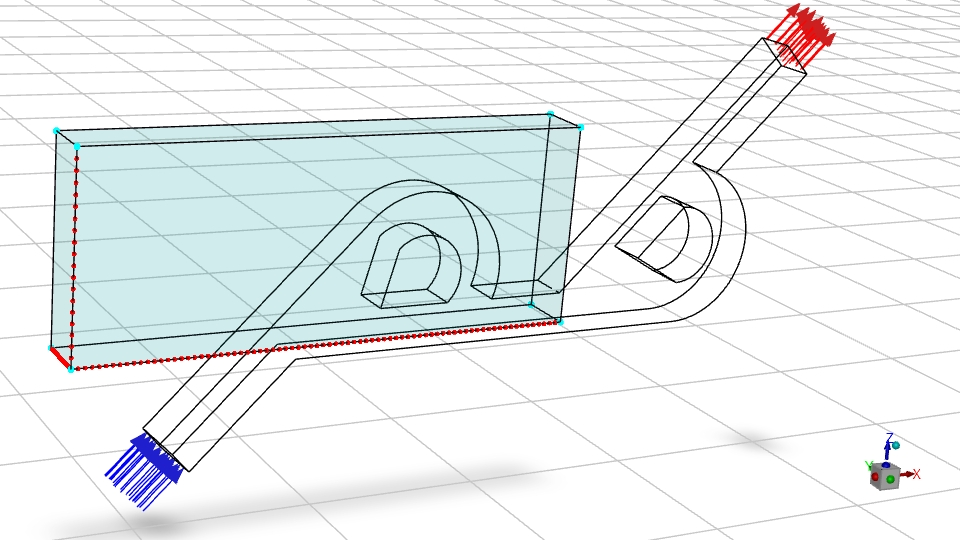
Case 1: Region is close to the boundaries, in your case it would be a narrow Z extent, for my case it's Y.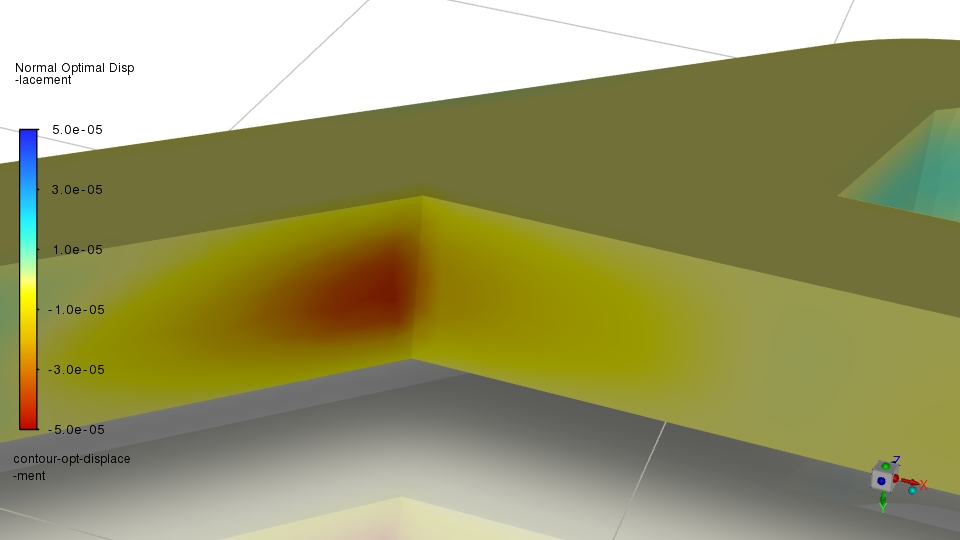

Case 2: Region has a distance of more than 2 control points (the red dots at the edges of the box) distance between the boundaries of the box and the geometry.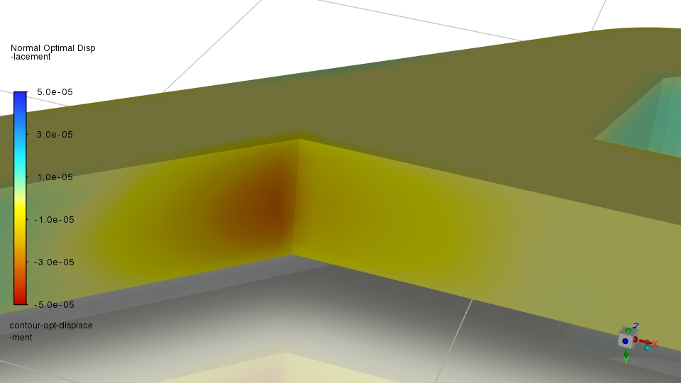

For both cases I do not allow deformation in that direction to ensure it stays within the bounds.

From the images you can see that the choice of the region changes how the model deforms. The expected deformation of the first case is focused in the center while the outer edges are not expected to move at all in both cases. After all, deformation in Y direction (up/down) is not possible here because of my user setting.
So, the definition of the region, the distribution of control points, and the morphing settings in general play a relevant role, not just the sensitivities. Even if you post all your settings, I cannot comment on all of them in the public forum. But I hope these hints help at least a little.

I also tried to run two optimizations with ten design iterations for my case. Target change is 5% reduction of the mass flow rate for each design change. I did this with two different regions, one that allows deformation of all surfaces and one that is focused just on the first bend.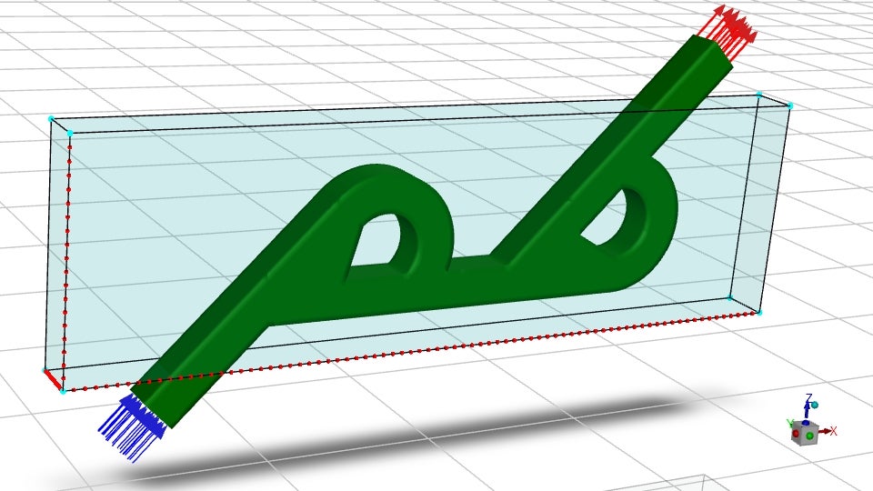

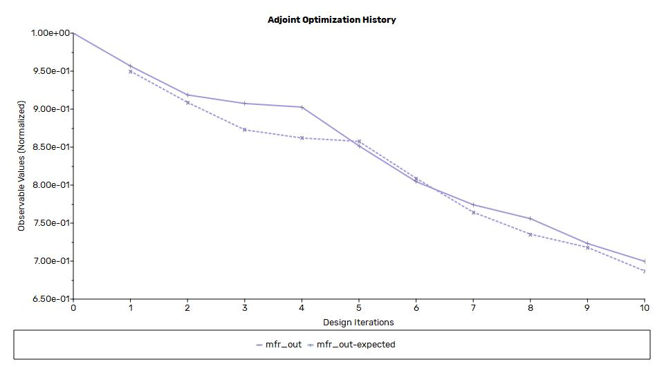
In my case there is a relevant deformation for both variations. My expectation was fulfilled that for the larger region the first edge is pushed inwards to choke the flow. That's not possible for the smaller region because this wall is outside the region. Since this high-sensitivity region is eliminated from deformation, other regions deform more, like the corner at the end of the bend.

Finally, regarding your question:
No, do not change the boundary conditions to amplify the flow. They should be realistic for your operating conditions. Changing the BCs can lead to a different 'optimal' result.
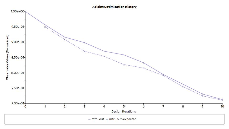
And no, do not amplify the deformation by increasing the target change value. There are times when this can help. But in your history plot you see that in the first step the expected change is very far from the achieved change. This means either your adjoint solution is poor or the change to the flow field is highly non-linear. Without understanding this first discrepancy, any brute force method will most likely fail, too.

What to do next?
Verify the flow field of the undeformed case. Do you have unexpected vortices? Double check material properties and domain size. Backflow can distrurb the flow field significantly. Verify that this does not interfere with deformable regions.
Can you figure out why the sensitivity plot is asymmetric and has such a high value in only one region? That might give you a hint why it deformes only there.
Check the region settings that you have enough space between the boundary and the geometry. From your screenshots it looks like you adjusted the number of control points already in the right direction. Verify, that there are more than two CPs between the boundary of the region and your walls.
Adjust the region to exclude the areas that should not deform. You can always run another set of design iterations with a different region in a second step.

[Jason Sum]

NA

[Akram Radwan]

Dear Jason,

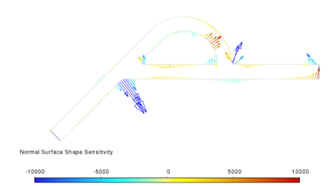
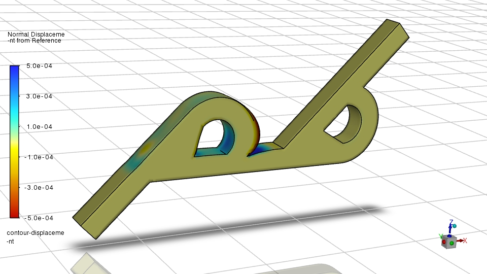
That sensitivity distribution looks a lot better than the one you shared earlier. It's unlikely that we get identical distribution. There are too many influence factors.

I can confirm the BCs. Pressure inlet on one side, pressure outlet on the other side. Observable is defined within the observable panel (not as expression) as integral of the mass flux on the inlet surface to have a positive sign without additional operations. Additionally, my test case uses a relatively low velocity with water and small dimensions. Therefore, I could run the case laminar. With a higher velocity it's challenging to converge the flow solver with respect to backflow in this flow direction without modifying the geometry.

[Jason Sum]

 

NA

[Jason Sum]

NA

[Jason Sum]

 

NA

[Rob]

Other than not using inflation, or rather getting the aspect ratio nearer 1.0 not really. If the separation or wake isn't stable convergence will be difficult. Most fluidic devices have local transient effects as they typically take advantage of "odd" fluid flow effects such as Coanda Effect. 

[Rob]

Yes, Akram's post got lost and he's a way for a week or two. He's aware of the site issues so will check on his return: we may need reminding given the number of threads! 

[Jason Sum]

Give that I already set the freefoam scale factor as 1, but still results similar to above. Or maybe sensitivity of outlet flow rate (observable) may not be that significant on the cells, which I may have to try select others as observables, such as velocity gradient of surface at recirculation regions, turbulence intensity at those regions? Or maybe combination of them by applying and trying different weightings of each? Is this normally the way I may go ahead to pursue a more effective morphing and enhancement in target? 

Thanks so much!