Learning Forum

[varunkash7]

I have been able to define a moving heat source using ACT extensions on ansys workbench. I happen to learn by reading some blogs that this is a gaussian heat source. However, I want to define a single point heat source as opposed to a path that is needed to be defined for a moving heat source. Is this possible?

I generated a function and applied it on the command module. However, this doesnt seem to work very well. Any thoughts? The code is attached. 

[varunkash7]

Hello? Can someone answer this for me please? When I contacted customer portal, I was asked to post my question here. It has been 2 weeks and no one has responded!

[Karthik Remella]

Hello,

Apologies for the delay. Could you please help us understand what you are modeling? Also, which tool are you using - Ansys Mechanical or Fluent to solve your problem? As Ansys employees, we cannot download any attachments. Please post screenshots here and we will be able to help you with your question.

Thanks.

Best,

Karthik

[varunkash7]

Hi Karthik,

Thanks for your response. I am modeling copper traces on a kapton (polyimide) sheet on Ansys mechanical. Im trying to simulate heat dissipation when a laser strikes the surface. The laser has a Gaussian heat profile. Therefore, I applied the ACT extension to obtain a moving Gaussian heat source to my model. However, this extension was not able to give me flexibility such as applying a point heat source with varying pulse rate etc. Therefore, I defined the Gaussian equation using function editor on Ansys mechanical APDL and used the attached code on the command module on Ansys mechanical. However, the equation in the command module is not being implemented. The code I am using to define a basic gaussian heat source is attached below

*SET,_FNCNAME,'Heatflux'

*DIM,_FNC_C1,,1 

*DIM,_FNC_C2,,1 

*DIM,_FNC_C3,,1 

*DIM,_FNC_C4,,1 

*SET,_FNC_C1(1),100 

*SET,_FNC_C2(1),46.19   

*SET,_FNC_C3(1),26.76   

*SET,_FNC_C4(1),0.08

*SET,_FNCCSYS,0 

! /INPUT,.DesktopHeatflux2.func,,,1   

*DIM,%_FNCNAME%,TABLE,6,19,1,,,,%_FNCCSYS%  

!   

! Begin of equation: B*exp(-1*(({X}/a)^2+({Y}/b)^2)/d^2)

*SET,%_FNCNAME%(0,0,1), 0.0, -999   

*SET,%_FNCNAME%(2,0,1), 0.0 

*SET,%_FNCNAME%(3,0,1), %_FNC_C1(1)%

*SET,%_FNCNAME%(4,0,1), %_FNC_C2(1)%

*SET,%_FNCNAME%(5,0,1), %_FNC_C3(1)%

*SET,%_FNCNAME%(6,0,1), %_FNC_C4(1)%

*SET,%_FNCNAME%(0,1,1), 1.0, -1, 0, 0, 0, 0, 0  

*SET,%_FNCNAME%(0,2,1), 0.0, -2, 0, 1, 0, 0, -1 

*SET,%_FNCNAME%(0,3,1),   0, -3, 0, 1, -1, 2, -2

*SET,%_FNCNAME%(0,4,1), 0.0, -1, 0, 1, 0, 0, -3 

*SET,%_FNCNAME%(0,5,1), 0.0, -2, 0, 1, -3, 3, -1

*SET,%_FNCNAME%(0,6,1), 0.0, -1, 0, 1, 2, 4, 18 

*SET,%_FNCNAME%(0,7,1), 0.0, -3, 0, 2, 0, 0, -1 

*SET,%_FNCNAME%(0,8,1), 0.0, -4, 0, 1, -1, 17, -3   

*SET,%_FNCNAME%(0,9,1), 0.0, -1, 0, 1, 3, 4, 19 

*SET,%_FNCNAME%(0,10,1), 0.0, -3, 0, 2, 0, 0, -1

*SET,%_FNCNAME%(0,11,1), 0.0, -5, 0, 1, -1, 17, -3  

*SET,%_FNCNAME%(0,12,1), 0.0, -1, 0, 1, -4, 1, -5   

*SET,%_FNCNAME%(0,13,1), 0.0, -3, 0, 1, -2, 3, -1   

*SET,%_FNCNAME%(0,14,1), 0.0, -1, 0, 2, 0, 0, 20

*SET,%_FNCNAME%(0,15,1), 0.0, -2, 0, 1, 20, 17, -1  

*SET,%_FNCNAME%(0,16,1), 0.0, -1, 0, 1, -3, 4, -2   

*SET,%_FNCNAME%(0,17,1), 0.0, -1, 7, 1, -1, 0, 0

*SET,%_FNCNAME%(0,18,1), 0.0, -2, 0, 1, 17, 3, -1   

*SET,%_FNCNAME%(0,19,1), 0.0, 99, 0, 1, -2, 0, 0

! End of equation: B*exp(-1*(({X}/a)^2+({Y}/b)^2)/d^2)  

!-->

sf,FACENAME,hflux,%Heatflux%  !FACENAME is named selection 

Here, B is the peak heat flux (i.e. the heat flux at the center {X}=0, {Y}=0), {X} and {Y} are the spatial coordinates and a, b, and d are scaling parameters for the size of the beam

I checked the coordinates to be global as well as defined in the above code.

Thanks for helping out with this.

Best,

Varun

[jrgv528]

Hi, what version are you using for?

[varunkash7]

Hi, I am using 19R2.

[Rohith Patchigolla]

Hi Varun, 

I tested your script on a 1x1 m^2 square plate in XY plane with centroid located at origin, in ANSYS Mechanical in v2019R2. 

The Heat flux applied looks like this picture below. 

 

So, it looks to be working (i.e. as a point source, with peak of 100 at center, i.e. X=0, Y=0).

Please let me know your comments on why you think it is not working at your end? Please check if you are using the correct units in Mechanical while solving, while the numbers in the command object will be interpreted in the solver unit system. 

Best regards,
Rohith

[varunkash]

Thanks for your reply Rohith. Yes, now on just using the equation without absorption coefficient it works fine. However, I am unable to modify the above equation with absorption coefficient as shown in the equation below, 

Here alpha is the absorption coefficient. It is a linear function of temperature. The earlier script contains the first part of the equation (without alpha). I even checked various commands under MP to see if it will let me define absorption coefficient. It does not contain such an option. Can you let me know how can I can incorporate this please?

 

Thank you.

Best,

Varun

[SteBir]

Hi varunkash7,

it's really easy to achieve this goal by using an APDL snippet. Check out these video links:

https://www.youtube.com/watch?v=DkAsSXdXG7I&list=PLzzqBYg7CbNqNlrA1QWayuhW_iEFpzCFH&index=3

https://www.youtube.com/watch?v=vQKoEDhFIsI&list=PLzzqBYg7CbNqNlrA1QWayuhW_iEFpzCFH&index=4

https://www.youtube.com/watch?v=NVXGFokDiRA&list=PLzzqBYg7CbNqNlrA1QWayuhW_iEFpzCFH&index=8

https://www.youtube.com/watch?v=UmT77Ro8u_Y&list=PLzzqBYg7CbNqNlrA1QWayuhW_iEFpzCFH&index=9

There you can see how to implement the moving heat source without ACT plugin.

Hope this helps you to achieve your goal

 

[varunkash7]

Hello! Thanks for your response. As I mentioned  when I initially posted the question, I already tried using the ACT plugin. The issue however is that this is not customizable based on the parameters I want to work with in my model. Everything is predefined. Moreover, there is a requirement to assign a path (since its a moving heat source) and I was unable to define a point Gaussian heat source using this.

Having said this, I want to define absorption coefficient as one of the influencing parameters using a APDL script. I have seen the videos you posted before. The issue is that these are all moving heat source models and if you see the equation used in the last video, it is a simplest form of the Gaussian equation with time dependency. It does not address the use of absorption coefficient. 

Therefore, just to reiterate my question, how do I incorporate absorption coefficient based on the earlier equation I posted using a APDL command?

Thanks,

[Rohith Patchigolla]

Hi Varun, 

Sorry for the delay. 

You mentioned earlier that the absorption coefficient, alpha is a linear function of temperature. You can incorporate this very easily while defining the function in the Function Editor in Mechanical APDL GUI. 

I tested a small example (i.e. using the below function in Mechanical via Command object) and it seems to work as expected (i.e. varies as a function of X, Y, Temp and Z). In the below example, I used alpha = 5*Temp (i.e. a linear function).

*DEL,_FNCNAME   
*DEL,_FNCMTID   
*DEL,_FNCCSYS   
*SET,_FNCNAME,'mytable' 
*SET,_FNCCSYS,0 
! /INPUT,myfunc.func,,,1
*DIM,%_FNCNAME%,TABLE,6,19,1,,,,%_FNCCSYS%  
!   
! Begin of equation: exp(-1*(({X}^2+{Y}^2)/2 - 5*{TEMP}*{Z}))   
*SET,%_FNCNAME%(0,0,1), 0.0, -999   
*SET,%_FNCNAME%(2,0,1), 0.0 
*SET,%_FNCNAME%(3,0,1), 0.0 
*SET,%_FNCNAME%(4,0,1), 0.0 
*SET,%_FNCNAME%(5,0,1), 0.0 
*SET,%_FNCNAME%(6,0,1), 0.0 
*SET,%_FNCNAME%(0,1,1), 1.0, -1, 0, 0, 0, 0, 0  
*SET,%_FNCNAME%(0,2,1), 0.0, -2, 0, 1, 0, 0, -1 
*SET,%_FNCNAME%(0,3,1),   0, -3, 0, 1, -1, 2, -2
*SET,%_FNCNAME%(0,4,1), 0.0, -1, 0, 1, 0, 0, -3 
*SET,%_FNCNAME%(0,5,1), 0.0, -2, 0, 1, -3, 3, -1
*SET,%_FNCNAME%(0,6,1), 0.0, -1, 0, 2, 0, 0, 2  
*SET,%_FNCNAME%(0,7,1), 0.0, -3, 0, 1, 2, 17, -1
*SET,%_FNCNAME%(0,8,1), 0.0, -1, 0, 2, 0, 0, 3  
*SET,%_FNCNAME%(0,9,1), 0.0, -4, 0, 1, 3, 17, -1
*SET,%_FNCNAME%(0,10,1), 0.0, -1, 0, 1, -3, 1, -4   
*SET,%_FNCNAME%(0,11,1), 0.0, -3, 0, 2, 0, 0, -1
*SET,%_FNCNAME%(0,12,1), 0.0, -4, 0, 1, -1, 4, -3   
*SET,%_FNCNAME%(0,13,1), 0.0, -1, 0, 5, 0, 0, 5 
*SET,%_FNCNAME%(0,14,1), 0.0, -3, 0, 1, -1, 3, 5
*SET,%_FNCNAME%(0,15,1), 0.0, -1, 0, 1, -3, 3, 4
*SET,%_FNCNAME%(0,16,1), 0.0, -3, 0, 1, -4, 2, -1   
*SET,%_FNCNAME%(0,17,1), 0.0, -1, 0, 1, -2, 3, -3   
*SET,%_FNCNAME%(0,18,1), 0.0, -1, 7, 1, -1, 0, 0
*SET,%_FNCNAME%(0,19,1), 0.0, 99, 0, 1, -1, 0, 0
! End of equation: exp(-1*(({X}^2+{Y}^2)/2 - 5*{TEMP}*{Z})) 
!-->

sf,myface,hflux,%mytable%

Please try this at your end and let me know if you have any questions. 

Best regards,

Rohith

[varunkash]

Hi Rohith,

Thanks for your response. I tried this. Although the code works in giving a Gaussian profile like before, the variation with respect to temperature doesnt seem to be reflected. I tried to vary the linear equation with different coefficients. All of them give the same profiles. Also, the profile remains the same with or without the incorporation of TEMP in the equation.

Also, can you let me know if this TEMP function takes in feedback from surface temperature?

Thanks.

Varun

[Rohith Patchigolla]

Hi Varun, 

Please note that the temperature effect is reflected only once a load step is completed. 

For example, in LS 1, Temp value is taken as "Initial Temperature" --> by default 22C. Then once the LS1 is solved and we move on to LS2, the Temp value is now taken as Temperature calculated at the end of LS1. As mentioned earlier, I have verified this on a simple model with two loadsteps. 

If you have only 1 load step, you cannot see the temperature effect we don't have access (by default) for temperature results at each substep. You can look into using USRCAL command to access these Temperatures at each substep, to get this effect. If not, to see the temperature effect, I would suggest to use multiple loadsteps, applying the heatflux using this function via Command object at each loadstep. 

Hope this clarifies. 

Best regards,

Rohith

[varunkash7]

Thanks Rohith. I did that, however it still doesn't reflect this accurately. The thickness of polyimide sheet I am using is around 20 microns. Analytical calculations tell me that the heat should penetrate through the material. However, I dont see this happening for such a small thickness along z axis. The screenshot is attached. Thank you for your help.

[Rohith Patchigolla]

Hi Varun, 

To understand this better, It would be helpful to know more about your model.

Could you please paste your final script being used (along with a snapshot of details box of command object), your model settings (analysis settings - num of steps, time step sizes, initial temperature), other loads and bcs (if any) and model view in XY plane.

Best regards,

Rohith 

[varunkash7]

Hi Rohith. Thanks for your response. So, I simplified my model to check this. RIght now, it is just a 20 micron sheet of polyimide (kapton) on which I apply a point Gaussian heat source. The final script I am using is below.

The snapshot of details box of command object can be seen below

On the analysis settings, the number of steps is 3, Each time step is 40 microseconds, total of 120 microseconds as seen below. Initial temperature is 22 deg Celsius. 

There are no other loads currently. Just convective boundary conditions on all walls. The model view in the XY plane is shown below.

Thanks for your help Rohith.

Best,

Varun

[varunkash7]

Here is the final script, sorry.

[Rohith Patchigolla]

Hi Varun, 

Thank you for providing me the details. Please paste the text of your script (instead of an image), so that I can test the same at my end on a simple case. 

Also, from your results, I see you are experiencing thermal undershoot i.e Initial temperature = 22 C, Min Temperauture at 120 microseconds = -32.23 C, which should not happen. 

Please have a look at Thermal analysis guide --> Specifiying load step options in ansys help 

Number of substeps per load step, or the time step size

A nonlinear analysis requires multiple substeps within each load step. By default, the program uses one substep per load step.

In regions of severe thermal gradients during a transient (e.g., surfaces of quenched bodies), there is a relationship between the largest element size in the direction of the heat flow and the smallest time step size that will yield good results. Using more elements for the same time step size will normally give better results, but using more substeps for the same mesh will often give worse results. When using automatic time stepping and elements with midside nodes (quadratic elements), ANSYS, Inc. recommends that you control the maximum time step size by the description of the loading input and define the minimum time step size (or maximum element size) based on the following relationship:

ITS = Δ2 / 4 α

The  Δ value is the conducting length of an element (along the direction of heat flow) in the expected highest temperature gradient. The  α value is the thermal diffusivity, given by k/ρC. The k value is the thermal conductivity, ρ is the mass density, and C is the specific heat.

If the above relationship ITS = Δ^2/(4*alpha) is violated when using elements with midside nodes, the program typically calculates unwanted oscillations and temperatures outside of the physically possible range. When using elements without midside nodes, the unwanted oscillations are unlikely to occur, and the above recommendation for the minimum time step can be considered somewhat conservative.

Hope this helps. 

Best regards,

Rohith

[varunkash]

Thanks Rohith. Here is the text of the script. 

*SET,_FNCNAME,'Heatflux'

*DIM,_FNC_C1,,1 

*DIM,_FNC_C2,,1 

*DIM,_FNC_C3,,1 

*DIM,_FNC_C4,,1 

*DIM,_FNC_C5,,1 

*SET,_FNC_C1(1),50000   

*SET,_FNC_C2(1),45.659  

*SET,_FNC_C3(1),24.768  

*SET,_FNC_C4(1),91.97

*SET,_FNC_C5(1),0   

*SET,_FNCCSYS,12 

! /INPUT,.DownloadsAbsorpti.func,,,1  

*DIM,%_FNCNAME%,TABLE,7,28,1,,,,%_FNCCSYS%  

!   

! Begin of equation: B*exp(-1*((({X}/a)^2+({Y}/b)^2)/(2*d)^2) - ((11000-10* 

! {TEMP})*({Z}/h))) 

*SET,%_FNCNAME%(0,0,1), 0.0, -999   

*SET,%_FNCNAME%(2,0,1), 0.0 

*SET,%_FNCNAME%(3,0,1), %_FNC_C1(1)%

*SET,%_FNCNAME%(4,0,1), %_FNC_C2(1)%

*SET,%_FNCNAME%(5,0,1), %_FNC_C3(1)%

*SET,%_FNCNAME%(6,0,1), %_FNC_C4(1)%

*SET,%_FNCNAME%(7,0,1), %_FNC_C5(1)%

*SET,%_FNCNAME%(0,1,1), 1.0, -1, 0, 0, 0, 0, 0  

*SET,%_FNCNAME%(0,2,1), 0.0, -2, 0, 1, 0, 0, -1 

*SET,%_FNCNAME%(0,3,1),   0, -3, 0, 1, -1, 2, -2

*SET,%_FNCNAME%(0,4,1), 0.0, -1, 0, 1, 0, 0, -3 

*SET,%_FNCNAME%(0,5,1), 0.0, -2, 0, 1, -3, 3, -1

*SET,%_FNCNAME%(0,6,1), 0.0, -1, 0, 1, 2, 4, 18 

*SET,%_FNCNAME%(0,7,1), 0.0, -3, 0, 2, 0, 0, -1 

*SET,%_FNCNAME%(0,8,1), 0.0, -4, 0, 1, -1, 17, -3   

*SET,%_FNCNAME%(0,9,1), 0.0, -1, 0, 1, 3, 4, 19 

*SET,%_FNCNAME%(0,10,1), 0.0, -3, 0, 2, 0, 0, -1

*SET,%_FNCNAME%(0,11,1), 0.0, -5, 0, 1, -1, 17, -3  

*SET,%_FNCNAME%(0,12,1), 0.0, -1, 0, 1, -4, 1, -5   

*SET,%_FNCNAME%(0,13,1), 0.0, -3, 0, 2, 0, 0, 20

*SET,%_FNCNAME%(0,14,1), 0.0, -4, 0, 1, -3, 3, 20   

*SET,%_FNCNAME%(0,15,1), 0.0, -3, 0, 2, 0, 0, -4

*SET,%_FNCNAME%(0,16,1), 0.0, -5, 0, 1, -4, 17, -3  

*SET,%_FNCNAME%(0,17,1), 0.0, -3, 0, 1, -1, 4, -5   

*SET,%_FNCNAME%(0,18,1), 0.0, -1, 0, 1, -2, 3, -3   

*SET,%_FNCNAME%(0,19,1), 0.0, -2, 0, 10, 0, 0, 5

*SET,%_FNCNAME%(0,20,1), 0.0, -3, 0, 1, -2, 3, 5

*SET,%_FNCNAME%(0,21,1), 0.0, -2, 0, 11000, 0, 0, -3

*SET,%_FNCNAME%(0,22,1), 0.0, -4, 0, 1, -2, 2, -3   

*SET,%_FNCNAME%(0,23,1), 0.0, -2, 0, 1, 4, 4, 21

*SET,%_FNCNAME%(0,24,1), 0.0, -3, 0, 1, -4, 3, -2   

*SET,%_FNCNAME%(0,25,1), 0.0, -2, 0, 1, -1, 2, -3   

*SET,%_FNCNAME%(0,26,1), 0.0, -1, 7, 1, -2, 0, 0

*SET,%_FNCNAME%(0,27,1), 0.0, -2, 0, 1, 17, 3, -1   

*SET,%_FNCNAME%(0,28,1), 0.0, 99, 0, 1, -2, 0, 0

! End of equation: B*exp(-1*((({X}/a)^2+({Y}/b)^2)/(2*d)^2) - ((11000-10*   

! {TEMP})*({Z}/h))) 

!-->

sf,face,hflux,%Heatflux%     

[varunkash]

Hi Rohith, I tried calculating and defining minimum time step size using this equation. However, I still see a similar trend. Is there something else I can try to rectify this?

Best,

Varun

[Rohith Patchigolla]

Hi Varun, 

Could you try re-running your model with linear elements instead of default (quadratic) and let me know the results?

Best regards,
Rohith

[SteBir]

I thought about the possibility to implement the absorption coefficient in a simple Ansys model and

and created a way to consider the absorption coefficient like in the equation beneath:

 

https://www.youtube.com/watch?v=SLZg9D2eBDM

Maybe this helps to solve the issues

[Sandipanbo]

Hi, I am trying to model a Gaussian moving heat source in Ansys Mechanical APDL.nThe heat source equation is:nQ= 1000*exp(-3*({X}^2+({Y}-0.05*{TIME})^2)/0.01^2)nThe plate is of size 4m x 4m.nInitial condition is T= 295K for the whole domain.nConvection boundary condition along the outer edges : h= 20; T-ambient=295Kn...I am attaching the APDL code. However, it is not showing any results. Please help......nn/PREP7nn!!!!!!!!!!!!!!!!!!!!!  ELEMENT TYPE AND MATERIAL PROPERTIES !!!!!!!!!!!!!!!!!!!nET,1,PLANE55nMPTEMP,,,,,,,,  nMPTEMP,1,0  nMPDATA,KXX,1,,20nMPTEMP,,,,,,,,  nMPTEMP,1,0  nMPDATA,C,1,,300  nMPTEMP,,,,,,,,  nMPTEMP,1,0  nMPDATA,DENS,1,,5000 nMPTEMP,,,,,,,,  nMPTEMP,1,0nn!!!!!!!!!!!!!!!!!!!!!!!  GEOMETRY AND MESHING !!!!!!!!!!!!!!!!!!!!!!!!!!!nRECTNG,-2,2,0,4,  !!!! dimensions of plate = 4m x 4mn*do,i,1,4,1 nLESIZE,i, , ,20, , , , ,1  !!!!! mesh size !!!!!!n*enddonamesh,1!!!!!!!!!!!!!!!!!!!! MOVING HEAT SOURCE - Gaussian !!!!!!!!!!!!!!!!!!!!!!!!n*DEL,_FNCNAME  n*DEL,_FNCMTID  n*DEL,_FNCCSYS  n*SET,_FNCNAME,'flux1'  n*SET,_FNCCSYS,0 n! /INPUT,htflx1.func,,,1n*DIM,%_FNCNAME%,TABLE,6,22,1,,,,%_FNCCSYS%  n!  n! Begin of equation: 1000*exp(-3*({X}^2+({Y}-0.05*{TIME})^2)/0.01^2)  !!!!! Gausssian heat source equation !!!!!!nn!!!!!!!!!!!!!!!!!!!!!!!!!!! initial position of heat source at x=0 and y=0), velocity = 0.05m/s !!!!!!!!!!!!!!!!!!!!!!!!!n!!!!!!!!!!!!! arc radius = 0.01 m !!!!!!!!!!!!!!!!!!!!!n!!!!! factor q0 = 1000 !!!!!!!!!!!!!!!!!!!!!!!!!!!!1nn*SET,%_FNCNAME%(0,0,1), 0.0, -999  n*SET,%_FNCNAME%(2,0,1), 0.0 n*SET,%_FNCNAME%(3,0,1), 0.0 n*SET,%_FNCNAME%(4,0,1), 0.0 n*SET,%_FNCNAME%(5,0,1), 0.0 n*SET,%_FNCNAME%(6,0,1), 0.0 n*SET,%_FNCNAME%(0,1,1), 1.0, -1, 0, 0, 0, 0, 0  n*SET,%_FNCNAME%(0,2,1), 0.0, -2, 0, 1, 0, 0, -1 n*SET,%_FNCNAME%(0,3,1),  0, -3, 0, 1, -1, 2, -2n*SET,%_FNCNAME%(0,4,1), 0.0, -1, 0, 3, 0, 0, -3 n*SET,%_FNCNAME%(0,5,1), 0.0, -2, 0, 1, -3, 3, -1n*SET,%_FNCNAME%(0,6,1), 0.0, -1, 0, 2, 0, 0, 2  n*SET,%_FNCNAME%(0,7,1), 0.0, -3, 0, 1, 2, 17, -1n*SET,%_FNCNAME%(0,8,1), 0.0, -1, 0, 0.05, 0, 0, 1  n*SET,%_FNCNAME%(0,9,1), 0.0, -4, 0, 1, -1, 3, 1 n*SET,%_FNCNAME%(0,10,1), 0.0, -1, 0, 1, 3, 2, -4n*SET,%_FNCNAME%(0,11,1), 0.0, -4, 0, 2, 0, 0, -1n*SET,%_FNCNAME%(0,12,1), 0.0, -5, 0, 1, -1, 17, -4  n*SET,%_FNCNAME%(0,13,1), 0.0, -1, 0, 1, -3, 1, -5  n*SET,%_FNCNAME%(0,14,1), 0.0, -3, 0, 1, -2, 3, -1  n*SET,%_FNCNAME%(0,15,1), 0.0, -1, 0, 0.01, 0, 0, 0  n*SET,%_FNCNAME%(0,16,1), 0.0, -2, 0, 2, 0, 0, -1n*SET,%_FNCNAME%(0,17,1), 0.0, -4, 0, 1, -1, 17, -2  n*SET,%_FNCNAME%(0,18,1), 0.0, -1, 0, 1, -3, 4, -4  n*SET,%_FNCNAME%(0,19,1), 0.0, -1, 7, 1, -1, 0, 0n*SET,%_FNCNAME%(0,20,1), 0.0, -2, 0, 1000, 0, 0, -1 n*SET,%_FNCNAME%(0,21,1), 0.0, -3, 0, 1, -2, 3, -1  n*SET,%_FNCNAME%(0,22,1), 0.0, 99, 0, 1, -3, 0, 0n! End of equation: 1000*exp(-3*({X}^2+({Y}-0.05*{TIME})^2)/0.01^2)  n!-->nFINISH /SOLn!*  nANTYPE,4n!*  nTRNOPT,FULL nLUMPM,0 !!!!!!!!!!!!!!!!!!!!!!!!! BOUNDARY CONDTIONS- CONVECTION (h=20, T-ambient = 295 K) !!!!!!!!!!!!!!!!!!!!!!!!!!!!!!!!!!!!!!n!!!!!!!!!!!!!!!!!!!!!!!!!  INITIAL TEMPERATURE=295 K  !!!!!!!!!!!!!!!!!!!!!!!!!!!!!!!!!!!!!!!!!!!!!!!!!!!!!!!!!nnFLST,2,4,4,ORDE,2  nFITEM,2,1  nFITEM,2,-4  n/GO n!*  nSFL,P51X,CONV,20, ,295, nFLST,2,1,5,ORDE,1  nFITEM,2,1  n/GO n!*  n!*  nSFA,P51X,1,HFLUX, %FLUX1%  nFLST,2,441,1,ORDE,2 nFITEM,2,1  nFITEM,2,-441nIC,P51X,TEMP,295,DELTIM,1,0,0nOUTRES,ERASEnOUTRES,ALL,ALL  nLNSRCH,1nTIME,80nn/STATUS,SOLUnSOLVE  nFINISH 

[Sebastiano Santarpia]

 

Great post.

 

[Divya yadav]

hii....can you help me in adding stationary gaussian heat source in ansys fluent.....i need to simulate it in 2D square with air as a fluid and observe the convection effect in it.

 

[ME23MTECH02002]

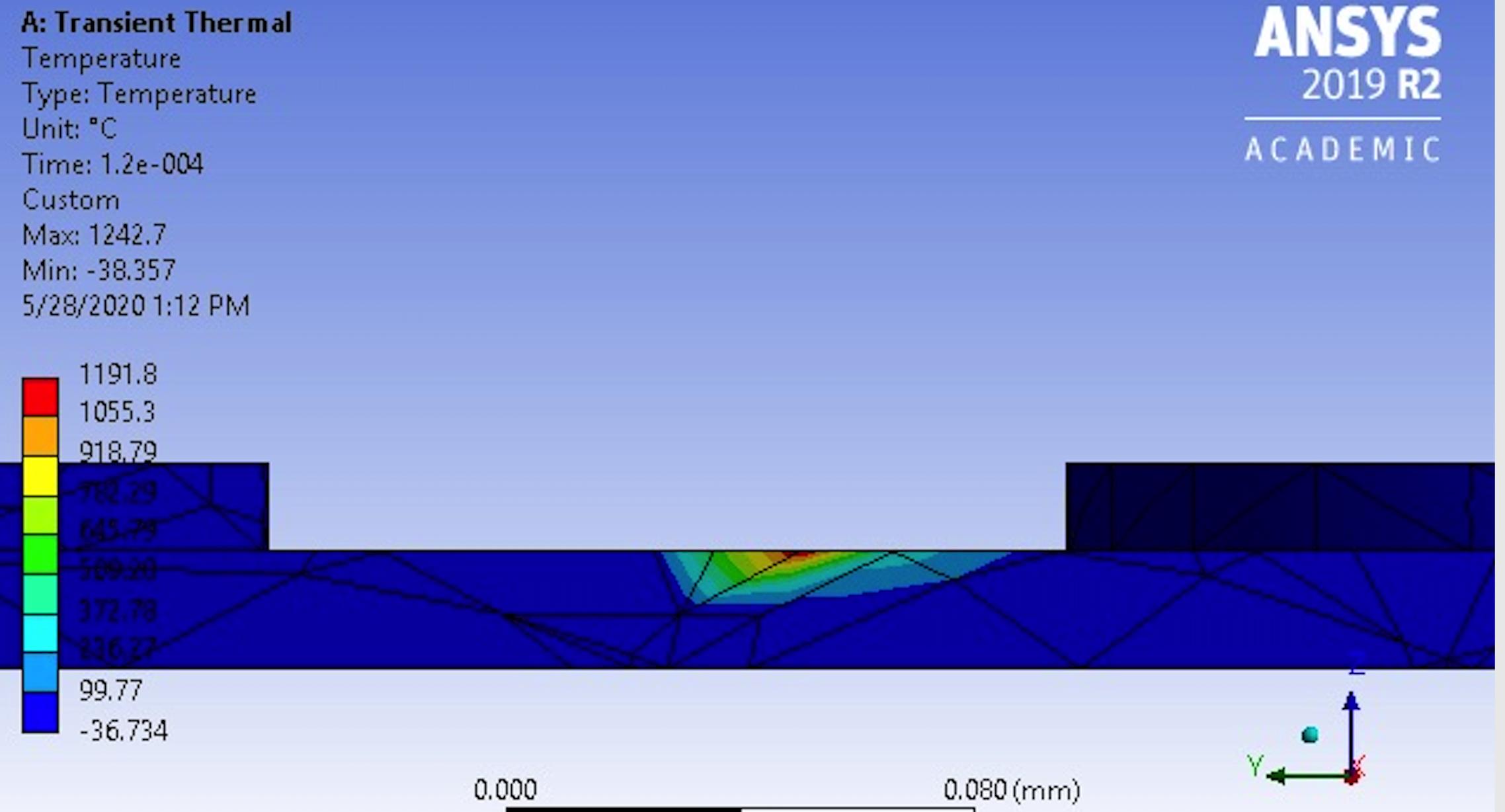
can anyone explain what the numbers in the row and columns of the heat flux table mean?

 

*SET,_FNCNAME,'Heatflux'

 

*DIM,_FNC_C1,,1 

 

*DIM,_FNC_C2,,1 

 

*DIM,_FNC_C3,,1 

 

*DIM,_FNC_C4,,1 

 

*DIM,_FNC_C5,,1 

 

*SET,_FNC_C1(1),50000   

 

*SET,_FNC_C2(1),45.659  

 

*SET,_FNC_C3(1),24.768  

 

*SET,_FNC_C4(1),91.97

 

*SET,_FNC_C5(1),0   

 

*SET,_FNCCSYS,12 

 

! /INPUT,.DownloadsAbsorpti.func,,,1  

 

*DIM,%_FNCNAME%,TABLE,7,28,1,,,,%_FNCCSYS%  

 

!   

 

! Begin of equation: B*exp(-1*((({X}/a)^2+({Y}/b)^2)/(2*d)^2) - ((11000-10* 

 

! {TEMP})*({Z}/h))) 

 

*SET,%_FNCNAME%(0,0,1), 0.0, -999   

 

*SET,%_FNCNAME%(2,0,1), 0.0 

 

*SET,%_FNCNAME%(3,0,1), %_FNC_C1(1)%

 

*SET,%_FNCNAME%(4,0,1), %_FNC_C2(1)%

 

*SET,%_FNCNAME%(5,0,1), %_FNC_C3(1)%

 

*SET,%_FNCNAME%(6,0,1), %_FNC_C4(1)%

 

*SET,%_FNCNAME%(7,0,1), %_FNC_C5(1)%

 

*SET,%_FNCNAME%(0,1,1), 1.0, -1, 0, 0, 0, 0, 0  

 

*SET,%_FNCNAME%(0,2,1), 0.0, -2, 0, 1, 0, 0, -1 

 

*SET,%_FNCNAME%(0,3,1),   0, -3, 0, 1, -1, 2, -2

 

*SET,%_FNCNAME%(0,4,1), 0.0, -1, 0, 1, 0, 0, -3 

 

*SET,%_FNCNAME%(0,5,1), 0.0, -2, 0, 1, -3, 3, -1

 

*SET,%_FNCNAME%(0,6,1), 0.0, -1, 0, 1, 2, 4, 18 

 

*SET,%_FNCNAME%(0,7,1), 0.0, -3, 0, 2, 0, 0, -1 

 

*SET,%_FNCNAME%(0,8,1), 0.0, -4, 0, 1, -1, 17, -3   

 

*SET,%_FNCNAME%(0,9,1), 0.0, -1, 0, 1, 3, 4, 19 

 

*SET,%_FNCNAME%(0,10,1), 0.0, -3, 0, 2, 0, 0, -1

 

*SET,%_FNCNAME%(0,11,1), 0.0, -5, 0, 1, -1, 17, -3  

 

*SET,%_FNCNAME%(0,12,1), 0.0, -1, 0, 1, -4, 1, -5   

 

*SET,%_FNCNAME%(0,13,1), 0.0, -3, 0, 2, 0, 0, 20

 

*SET,%_FNCNAME%(0,14,1), 0.0, -4, 0, 1, -3, 3, 20   

 

*SET,%_FNCNAME%(0,15,1), 0.0, -3, 0, 2, 0, 0, -4

 

*SET,%_FNCNAME%(0,16,1), 0.0, -5, 0, 1, -4, 17, -3  

 

*SET,%_FNCNAME%(0,17,1), 0.0, -3, 0, 1, -1, 4, -5   

 

*SET,%_FNCNAME%(0,18,1), 0.0, -1, 0, 1, -2, 3, -3   

 

*SET,%_FNCNAME%(0,19,1), 0.0, -2, 0, 10, 0, 0, 5

 

*SET,%_FNCNAME%(0,20,1), 0.0, -3, 0, 1, -2, 3, 5

 

*SET,%_FNCNAME%(0,21,1), 0.0, -2, 0, 11000, 0, 0, -3

 

*SET,%_FNCNAME%(0,22,1), 0.0, -4, 0, 1, -2, 2, -3   

 

*SET,%_FNCNAME%(0,23,1), 0.0, -2, 0, 1, 4, 4, 21

 

*SET,%_FNCNAME%(0,24,1), 0.0, -3, 0, 1, -4, 3, -2   

 

*SET,%_FNCNAME%(0,25,1), 0.0, -2, 0, 1, -1, 2, -3   

 

*SET,%_FNCNAME%(0,26,1), 0.0, -1, 7, 1, -2, 0, 0

 

*SET,%_FNCNAME%(0,27,1), 0.0, -2, 0, 1, 17, 3, -1   

 

*SET,%_FNCNAME%(0,28,1), 0.0, 99, 0, 1, -2, 0, 0

 

! End of equation: B*exp(-1*((({X}/a)^2+({Y}/b)^2)/(2*d)^2) - ((11000-10*   

 

! {TEMP})*({Z}/h))) 

 

!-->

 

sf,face,hflux,%Heatflux%