Pre-Analysis and Start-Up
Pre-Analysis
In the Pre-Analysis step, we'll review the following:
- Mathematical model: We'll look at the governing equations + boundary conditions and the assumptions contained within this complex nonlinear mathematical model.
- Numerical solution procedure in Ansys: We'll briefly overview the solution strategy used by Ansys to solve a nonlinear problem, with both a material nonlinearity as well as a contact nonlinearity.
- Hand-calculations of expected results: We'll use our intuition of mechanics and knowledge of the mathematical model to predict the expected solutions from Ansys. We'll pay close attention to additional assumptions that have to be made in order to obtain an analytical solution.
Mathematical Model
Here, looking at the governing equations, we have to evaluate what happens by adding material and contact nonlinearities into the model.
To start, looking at the 3D equilibrium equations, we will still have the equilibrium of an infinitesimal element, with F=ma=0, and no body forces applied. Thus, the differential equations of equilibrium remain the same.
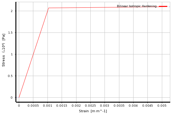
The material properties, however, now contain a nonlinearity. This occurs through a Bilinear Isotropic material property, which allows plastic deformation within the solution by creating a stress-strain curve that has two regions of different moduli;

With this, we now have an elastic modulus (E) that is dependent on the value of strain, and it can be either the first modulus or the second depending on the value of strain. In the 3D Hooke's Law;

we would then change the E into a function based on strain.
Similarly, we would also expect a change to occur in the Strain-Displacement relations below;

For more information on how contact changes the Mathematical Model of the problem, see Module 3 in our simulations MOOC at edx.org.
Numerical Solution Procedure in Ansys
Note that in large deflection problems, you need to tell Ansys to split load into increments (substeps). Ansys will iterate within each increment to solve the nonlinear algebraic equations that come from discretizing the governing equations.
For more information on how contact changes the Numerical Solution of the problem, again see Module 3 in our simulations MOOC at edx.org.
Hand-Calculations of Expected Results
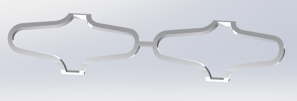
Due to the complexities in the model, we can't do any easy hand-calculations to find out what we'd expect to see, but we can still use the boundary conditions of the problem and what we know from our intuition to figure out what trends we'd expect to see. Looking at a quarter (symmetric) section of the model, we can imagine what would happen if the stent was expanded;

We know intuitively that if we expand the stent from the inside, we would expect the total length of the stent (from tip to tip) to decrease. How can we expect this displacement to effect stresses inside the body? For instance, we can expect higher stresses located in the curves of the model than we would see in the linear portions, due to the moments that the displacement will cause.
