
Tagged:
-
-
October 1, 2025 at 10:58 am
 FAQParticipant
 Table of contents
Introduction
FAQs
- What are the requirements to run Mechanical APDL solvers on GPUs?
- How do I choose GPU cards that work for me?
- Which GPU cards are recommended for use with Mechanical APDL’s GPU acceleration?
- I have a recommended card. Why won’t the software let me use it?
- What happens if I use a card that isn’t recommended?
- What about consumer-grade gaming cards?
- Which GPU configuration will deliver the best return for my workloads?
PrefaceIn recent years, graphics processing units (GPUs) have seen substantial hardware improvements, largely driven by investments in artificial intelligence (AI). The Mechanical APDL™ application has supported the use of GPUs to speed up finite element analysis (FEA) solutions since 2010. The newest cards are faster and larger than ever before, enabling the Mechanical APDL software to continue pushing the limits of model size and performance gain. However, with dozens of GPUs on the market for gaming, desktops, workstations, and large servers, it is more difficult than ever to select a GPU. This article covers:
- Key GPU features for accelerating FEA solutions
- Types of Mechanical APDL equation solvers
- Differences between Mechanical APDL solvers
- Top-performing GPUs for each solver

Figure 1: Technicians managing server infrastructure
IntroductionTo start, it is helpful to clarify the distinction between the Mechanical™ structural finite element analysis software and the Mechanical APDL application, along with the meaning of solvers and acceleration. The Mechanical software is a pre- and post-processor for structural analysis that generates input files for the Mechanical APDL application. Therefore, simulations run in the Mechanical APDL application inherently include those started from the Mechanical software.
The Mechanical APDL application is a pre- and post-processor with a variety of FEA solvers. The equation solvers can be broadly categorized as sparse direct solvers (often called just “sparse” or “direct”) and iterative solvers (commonly referred to as the PCG solver, though there are several available iterative solvers). A new mixed solver was recently introduced, blending aspects of both the direct and iterative solvers. This differentiates the Mechanical APDL application from other products that have only one type of solver. Since Mechanical APDL software includes multiple solvers, references are made to the category or type of solver instead of a specific name (for instance, preconditioned conjugate gradient versus Jacobian conjugate gradient; two iterative solvers).
GPU acceleration refers to transferring simulation data from the CPU to the GPU, specifically in the solution phase of an analysis. The Mechanical APDL application existed before multi-core CPU hardware was commonplace. Naturally, the software is primarily written for CPUs, even though much of it has been parallelized. The GPU hardware is designed to be exceptionally fast when handling parallel computational tasks, and this is what makes it attractive for speeding up solutions. Hence, when referring to a speedup, it means speeding up the solution. Other phases of an analysis, such as pre- and post-processing, are not considered.
Before proceeding, it is important to clarify several key distinctions between CPUs and GPUs.
1. What are CPUs?
Modern central processing units (CPUs) have flexible cores that can handle complex instruction sets. Typically, CPUs range from around 8-12 cores for desktop processors and up to 192 cores for the largest server processors. They are designed to handle a diverse set of tasks, from interfacing with hardware peripherals to the serious number crunching required by simulations. Modern CPUs can maintain a very high single-core clock speed (or frequency), which leads to faster computations, particularly for direct solvers. To achieve this high clock speed, CPUs are rated for increasingly high thermal design power (TDP) values, specified in watts. However, these high TDP values result in an overall reduction in clock speed as more cores are employed for parallel computations due to the heat generated. In terms of performance, clock speed is not the only factor to consider. Another key hardware metric is memory bandwidth. This is a measure of how fast the CPU cores can move data in and out of random-access memory (RAM, or just memory). With the kind of computations required by iterative solvers, memory bandwidth on a single machine can often become “saturated” before all the available CPU cores are used, and using more CPU cores will not lead to a faster solution.
2. What are GPUs?
Compared to CPUs, GPUs deliver much higher memory bandwidth and computational speed by using different groupings of specialized cores and high-bandwidth memory, resulting in significantly faster simulations. However, the process of transferring data to and from a GPU can diminish the overall performance gains. Therefore, it is important to carefully consider when and how to use a GPU to accelerate the solution.
GPUs excel in several categories of computation, some of which are specialized:
- FP32 – single precision floating point calculations
- FP64 – double precision floating point calculations
- Tensor cores – accelerated matrix/vector operations
- Ray tracing cores – calculation of rays emitted from an object to an observer
These different types of computations are what set GPUs apart in their application. A gaming GPU might be packed with ray tracing cores but have very little (or no) FP64 capabilities. On the other hand, high-end server GPUs may not have any ray tracing cores at all but have significant FP32 and FP64 performance. Therefore, a gaming GPU would be a poor candidate for speeding up FEA simulation, while a server GPU would perform poorly in gaming.
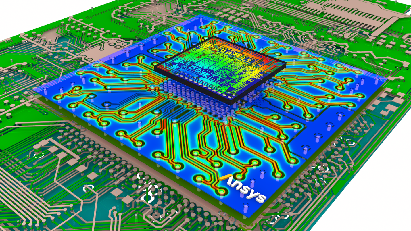
Figure 2: Simulation of microchip using Ansys software
3. Using GPUs with the Mechanical APDL solvers
Simulations in the Mechanical APDL application make use of a variety of equation solvers, but the most used is either a sparse direct solver or an iterative solver, both of which compute the solution in double precision (FP64).
Although both solvers have their own strengths, the iterative solver works especially well with GPUs. This solver is memory-bandwidth bound, meaning its performance depends on how quickly data moves between memory and the processor. Higher memory bandwidth leads to faster solver performance. Since GPUs offer significantly more bandwidth than CPUs, they deliver greater speedup when running iterative solvers.
The sparse direct solver is compute-bound, meaning that it is limited by the clock speed of a CPU. This makes significant FP64 rates a requirement for accelerating the sparse solver on GPUs.
The mixed solver, a recent introduction to the Mechanical APDL application, uses principles and technology from both the direct and iterative solvers to reduce overall memory, maintain high accuracy, and achieve better performance on GPUs that have only high single-precision (FP32) compute rates.
4. Good news and bad news
Many of the less expensive GPU cards have little or no FP64 computational speed at all. This includes workstation cards like the Nvidia RTX Ada series and the new RTX Pro cards. It also includes cards like the Nvidia A10 and L40 server-class cards. It is only the especially high-end cards that have high FP64 compute rates, such as the Nvidia A100/H100/H200/B100 or AMD MI200/210/300x Instinct cards. This is the “bad” news, in the sense that the highest-end cards are prohibitively expensive, and often difficult to source.
The good news is that the most widely used Mechanical APDL application solvers support GPU cards across a range of price points, enabling simulations to benefit from enhanced performance with a more moderate financial outlay.
The following benchmark comparison illustrates how GPUs can perform in Mechanical APDL workloads (Benchmark Mechanical Information | Ansys). For this direct solver benchmark model in the V25 set, an Nvidia H100 GPU provides consistent acceleration compared to running with only CPU cores.
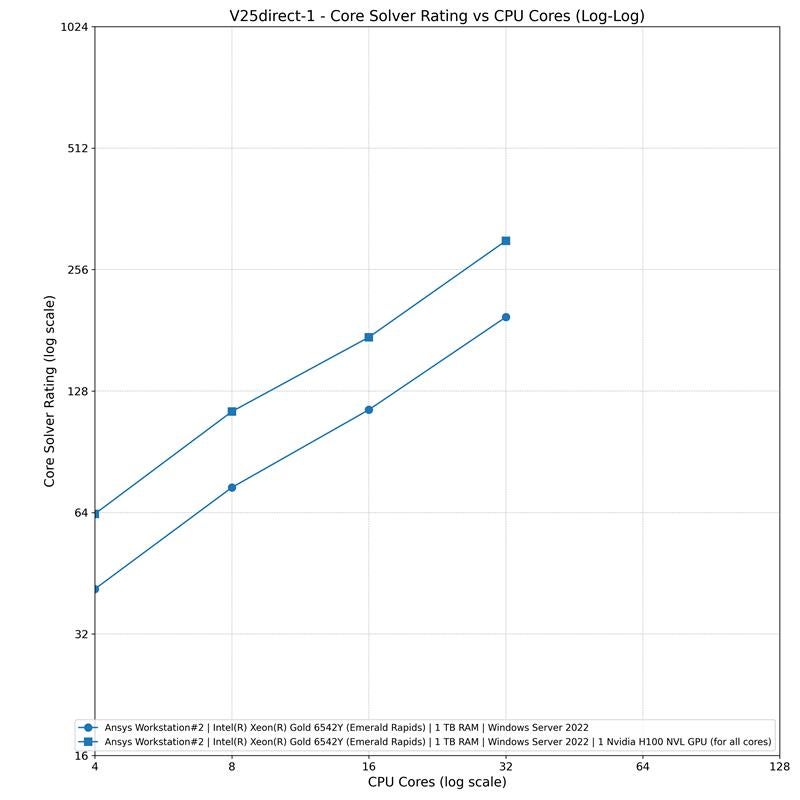
Figure 3: CPU versus GPU performance for a direct solver benchmark
FAQs1. What are the requirements to run Mechanical APDL solvers on GPUs?
General requirements:
- Run on Windows 64-bit or Linux x64 platforms.
- Simulation must have a supported analysis type with supported features.
- Almost all features are supported except for partial pivoting with the sparse solver, commonly used for mixed u-P elements, Lagrange multiplier MPC184 (joint) elements or contact elements, and certain circuit elements.
- Use a GPU device recommended for your solver choice.
- Have adequate licenses. The Mechanical APDL licenses cores and GPUs, not GPU multiprocessors. Using the baseline four cores/GPUs, you can make combinations like these:
- four CPU cores
- two CPU cores and two GPU cards
- Activate the GPU acceleration option through either of the two methods:
-
- In the Mechanical APDL Product Launcher, select the High-Performance Computing Setup tab, choose the appropriate GPU Acceleration option from the dropdown, and specify the number of GPUs to use during the solution.
-
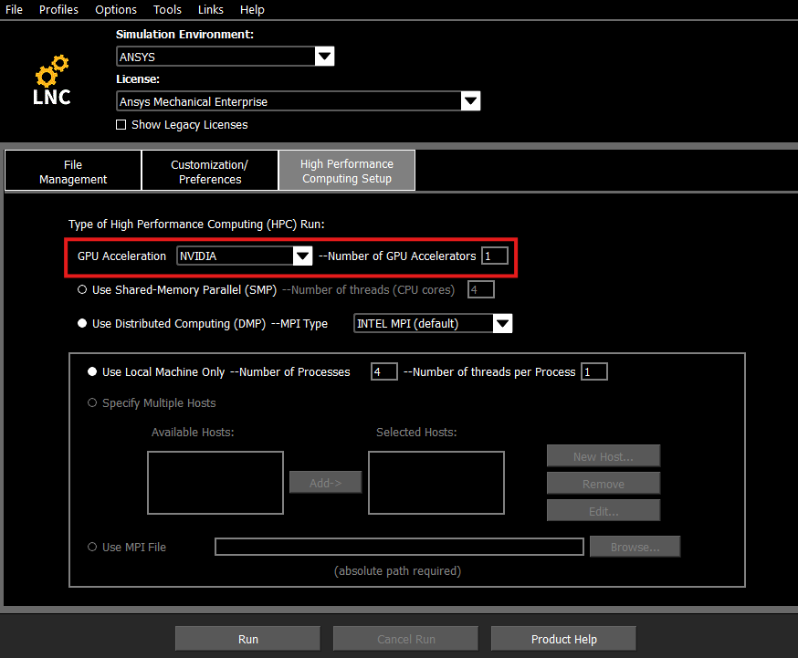
Figure 4: Activate GPU acceleration through the Product Launcher
-
- Or, as a command line argument.
For example, with one NVIDIA GPU: ansys252 -acc nvidia -na 1
Or with two AMD GPUs (Linux only): ansys252 -acc amd -na 2
- Or, as a command line argument.
2. How do I choose GPU cards that work for me?
This is the most pressing question. Ask yourself the following:
- What type of solver do you use (or require)?
- What is the size of your model?
- What is your budget?
Key GPU Specifications for Equation Solver Performance
GPU data sheets often include extensive technical details. To assess performance for solver workloads, focus on these four key specifications:
- FP64 performance (FLOPS): Measures the speed of double-precision calculations, which directly impacts the performance of the direct solver.
- FP32 performance (FLOPS): Indicates how fast single-precision calculations are performed. This is especially relevant for mixed solver performance.
- GPU memory bandwidth (TB/s): Higher bandwidth enables faster data transfers, benefiting all solver types, especially the iterative solver.
- GPU memory capacity (GB): Larger memory enables more computations to be offloaded to the GPU, enhancing overall solver efficiency.
Equation Solver Type
If your model requires the sparse solver, then only the highest-end GPUs are recommended to speed up the simulation. If you cannot afford the high price tag of the largest GPUs, the mixed solver might work on a lower-end card. If your model runs well with the iterative solver, then virtually any of the recommended GPU cards will work.
Model Size
Model size, particularly in terms of memory requirements, is a challenging metric to estimate in advance. The relationship between GPU capacity and model size is especially relevant when using the PCG solver.
For the Mechanical APDL application, offloading the iterative solution to the GPU is typically an “all or nothing” process. If the model exceeds the available GPU memory, the solution cannot be offloaded.
If you have some simulations you run on a regular basis that use the PCG solver, check the *.PCS file for Memory Usage for Matrix. It is difficult to state a hard and fast rule-of-thumb, but around 1.5x this number might give an approximate size of the minimum GPU memory your simulation requires.
To apply this guidance, consider the following example using one of the previous hardware benchmark models from the V24 Mechanical application. The V24 iter-1 benchmark (Benchmark Mechanical Information | Ansys) uses the PCG solver, has a symmetric matrix, 23.3 million degrees of freedom (MDOF), and conducts a static, linear, structural analysis.
The degrees of freedom can be estimated by multiplying the number of nodes by their respective number of DOF (three for solid elements, six for beams/shells).
The *.PCS file contains the following memory statistics (2025R2, DMP -np 4):
Parameter Value Total Memory Usage at CG 36.51 GB PCG Memory Usage at CG 16.17 GB Memory Usage for Matrix 11.11 GB Applying the estimates, the anticipated memory need is 1.5 x 11GB = 16.5GB. To be conservative, a GPU with a minimum of 24GB of memory would be an appropriate choice.
In contrast with the PCG solver, the sparse direct solver has an optimal range of calculations that can use the GPU to speed up the solution. Calculations that are too big simply won’t fit on the GPU, and calculations that are too small may be faster to solve on the CPU. Because of this, it is difficult to predict exactly how much a GPU will accelerate a solution before running it. When using a GPU with the sparse direct solver, a statistic of what percentage of calculations were offloaded to the GPU is printed in the *.DSP file after a run. Low percentages, such as 50-75%, indicate that the model and GPU pair are not well matched.
Lastly, budget plays an enormous role in deciding what GPUs are worth considering. Before purchasing a GPU, consider renting time on cloud resources to benchmark your model with GPUs. If you see significant speedup, there may be value in purchasing the same card. Or, if you only occasionally need to use a GPU, continuing to pay-as-you-go for cloud hardware could be the best value. Inquire about the Ansys Gateway powered by AWS and Ansys Access powered by Azure offerings if you are seriously considering augmenting your resources with a cloud computing approach.
For more plots comparing GPU and CPU hardware, check out the benchmark results Ansys publishes on different hardware: Benchmark Mechanical Information | Ansys. If your simulation is similar to one of the standard benchmarks, that might be a clue for what hardware could work.
3. Which GPU cards are recommended for use with Mechanical APDL GPU acceleration?
A list of tested hardware for the different Ansys products is available here: Platform Support and Recommendations | Ansys.
The Mechanical APDL application is tested and verified with all the following Nvidia and AMD GPU cards:
- Workstation: RTX A4000, RTX A5000, RTX A6000, RTX A6000 Ada, Quadro RTX 6000
- PROS: Typically, these cards are affordable and readily available for purchase. They can be used for many other applications, including high-end visualization.
- CONS: Only well-suited for iterative and mixed solvers, and memory capacity is limited.
- Server: A100, H100, Instinct MI210
- PROS: Highest-end GPU cards that will benefit virtually all simulations.
- CONS: The cards are expensive and can be difficult to obtain.
- Server: A40, L40
-
- PROS: Performance and price are slightly above the high-end workstation cards but much lower than the high-end server cards. For iterative solvers they remain a good choice.
- CONS: Like the workstation cards, these are only well-suited for iterative solvers and have limited memory capacity.
-
The Mechanical APDL application supports many more GPU cards than those mentioned above. It is recommended that you benchmark your GPU cards to find the best one for your application.
4. I have a recommended card. Why won’t the software let me use it?
If you have an older version of the software and a newer card, you might be blocked from using that card since the older software does not recognize the card. You can override this block and proceed if the card is on the recommended list in a recent release.
5. What happens if I use a card that isn’t recommended?
Cards that are not recommended at all can be separated from those that are recommended for only one solver.
If a card is not recommended at all, the Mechanical APDL application will prevent you from using it by default. Your specific simulation and specific GPU might provide a speedup, but it can also cause a simulation to run more slowly. The block can be overridden, as explained in the documentation (Linux and Windows). This behavior acts as a guardrail to prevent poorly performing cards from degrading solution performance versus running solely on CPU cores.
In the latter case, if you are using a card that is recommended for the iterative solver, and run your solution with the sparse direct solver, then the Mechanical APDL application will respect that choice and proceed with the solution. However, you may not see any speed up, and in some cases, will see a reduction in performance.
6. What about consumer-grade gaming cards?
These cards have historically lacked the performance to offer a meaningful speedup and therefore are not recommended or tested with the Mechanical APDL application.
7. Which GPU configuration will deliver the best return for my workloads?
The best GPU configuration depends on your specific Mechanical APDL workloads, including model size, solver type, memory requirements, and how often you run GPU-accelerated analyses. There is no single best GPU for all use cases.
Ansys provides the GPU ROI Estimator to help estimate the return on investment for your environment. The estimator evaluates expected performance improvements and cost efficiency based on your workloads.
For additional background and guidance, see the Ansys blog post Introducing the GPU ROI Estimator Tool for Fluent, Mechanical Software.
-


Introducing Ansys Electronics Desktop on Ansys Cloud
The Watch & Learn video article provides an overview of cloud computing from Electronics Desktop and details the product licenses and subscriptions to ANSYS Cloud Service that are...
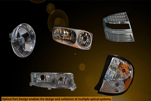
How to Create a Reflector for a Center High-Mounted Stop Lamp (CHMSL)
This video article demonstrates how to create a reflector for a center high-mounted stop lamp. Optical Part design in Ansys SPEOS enables the design and validation of multiple...
Introducing the GEKO Turbulence Model in Ansys Fluent
The GEKO (GEneralized K-Omega) turbulence model offers a flexible, robust, general-purpose approach to RANS turbulence modeling. Introducing 2 videos: Part 1 provides background information on the model and a...
Postprocessing on Ansys EnSight
This video demonstrates exporting data from Fluent in EnSight Case Gold format, and it reviews the basic postprocessing capabilities of EnSight.

- How do I request ANSYS Mechanical to use more number of cores for solution?
- How to restore the corrupted project in ANSYS Workbench?
- What is the reason for this error message when mesher fails – “A software execution error occurred inside the mesher. The process suffered an unhandled exception or ran out of usable memory.”?
- Contact Definitions in ANSYS Workbench Mechanical
- How can I change the background color, font size settings of the avi animation exported from Mechanical? How can I improve the resolution of the video?
- How to transfer a material model(s) from one Analysis system to another within Workbench?
- There is a unit systems mismatch between the environments involved in the solution.
- How to deal with “”Problem terminated — energy error too large””?”
- How to change color for each body in Mechanical?
- How can I recover results from other previously solved analyses in the Workbench project?

© 2026 Copyright ANSYS, Inc. All rights reserved.
