Learning Forum

[vladr]

Dear Forum Members,

I am setting up a model of directional solidification (crystal growth) with chemical species transport. The objective is to model solidification of an ingot and obtain a solute distribution profile in the final solid along the freezing direction. In the final model the convection in the melt will need to be included, however at this stage I am trying to debug the model that only accounts for Temperature, Solidification and Species with the momentum equations turned off.

The situation that I am trying to replicate is a theoretical model of "Diffusion-Controlled 1-dimensional solidification" that occurs when a pool of molten material with evenly distributed solute is frozen by moving it with respect to a 1-D temperature gradient, without convection in the liquid phase (melt) and without diffusion in the solid phase (crystal or ingot). As the temperature decreases, the material starts to solidify at one end, and the solute is partially incorporated into the solid and partially rejected. This results in a solute concentration in the first bits in the solid lower than initial, and a build up of the concentration in the liquid next to the solid-liquid interface, due to limited solute transfer into the bulk liquid by diffusion. The build-up continues until the rate of the solute rejection at the interface is balanced by the rate of its transfer away by diffusion. In a final solid bar this process produces an "initial transient" of increasing concentration followed by a "steady-state" section, which is described by a picture below.

[Surya Deb]

Hello, nI am trying to understand your problem in a better way. I understand that you don't want to have a wide range of solidification temperature and want to have the Tliquidus and Tsolidus very close to each other. nIs the problem now with convergence as you mentioned after a few time steps?nHow does the Temperature field look like and could you also check the mass diffusivity of the species that you are using?nDo you take this diffusivity value from experimental/test data?nRegards,nSuryann

[vladr]

Dear Surya,nthanks a lot for your reply.nnFirst thing, to clarify better what am I trying to do: nnIdeally I would like to completely decouple the Temperature, Convection and Solidification from the Species Concentration. I.e. to have a problem of a solidifying pure material (InSb) with a single melting Temperature, without (or with minimal) 2-plase mushy zone, and to have the Species field as a Passive Scalar.nFrom playing previously with a pure material solidification problem I know that I still need (for some reason) to have Tsolidus and Tliquidus, which I made 0.0001 K apart, but still had a small mushy zone region. If there's no good workaround, I can live with that, provided that the mushy zone does not influence melt convection and convection-diffusion of the solute in the melt.nImportantly, I'd like to have the Species Concentration as a passive scalar field that obeys: n1) The partial rejection of the solute at the solid-liquid interface into the liquid and partial incorporation of it into the formed solid, that would be determined by the partition coefficient K;n2) Convection-Diffusion for the solute that's in the liquid (without solutal buoyancy) n3) No diffusion for the solute in the formed solid, so that once its in the solid it does not redistribute itself along the solid.nIdeally, I would also like not to have any mushy zone, like it is a sharp interface, to model the convective field/boundary layer at the interface influence on the solute incorporation in the formed solid. But for now I leave this question out, because at this stage I am trying to properly duplicate the diffusion controlled scenario described above (and to verify it with analytical solution). Though, I am also concerned with the mushy zone influencing the diffusion of of the solute away from the build-up region next to the interface, that may get in the way of matching the analytical solution, so If you can shed some light on it for me I would appreciate it.nnI would very much welcome any suggestions on if there is a better (more robust and less expensive) way to set this up compared to how I did it.nnNo to the answers to the rest of your questions:nnIs the problem now with convergence as you mentioned after a few time steps?nIt went like this: I would start the calculation in the evening and monitor the first few hundred timesteps, it would start by easily hitting the residual in few iterations, then after a few timesteps (probably when the solidification starts to progress) it would start to struggle to hit the prescribed concentration residual (10^-, though still coming pretty close to it in few iterations, while the temperature is doing OK. Then I would decrease the timestep and it starts to converge in few iterations again, and I leave it over night. nBut when I look at it the next day (when its already at ~80% of the process) I find that C residual does not fall much below 10^-3 in the prescribed iteration limit (100-200), it kind off levels out. The temperature residual is doing better, it still is much worse compared to what I prescribe (like 10^-6 instead to 10^-9). Unfortunately I was not saving the whole history to see when it starts to go wrong, I only could see this from the iterations displayed in the plot/terminal for the last stages of the computation. All this is speaking of the more problematic case (slower freezing, 2mm/hr). nFor the the less problematic one (faster freezing 1cm/hr) I think I was finding it doing OK on the last stages in the late stages of the process, but the concentration plot would display that the Initial Transient stage did not go well (the left side of the color plot and the first chart above).nnHow does the Temperature field look like?nFor the more successful (1 cm/hr) case the temperature field looks ok including the early phase (10 min into the process) resulting in problematic concentration section, see the plots below:nnnCould you also check the mass diffusivity of the species that you are using?nI am using the diffusion coefficient 10^-9 (m^2/s) for the solute (Te), and because I am using the dilute model I think its irrelevant for the Solvent.nnDo you take this diffusivity value from experimental/test data?nI took this value from the following paper:nModel of Tellurium- and Zinc-Doped Indium Antimonide Solidification in Space, Alexei V. Churilov and Aleksandar G. Ostrogorsky, Journal of Thermophysics and Heat Transfer 2005 19:4, 542-547, https://arc.aiaa.org/doi/10.2514/1.8463nThat in its turn is referencing the experiemtnally measured value reported here:nAleksandar G. Ostrogorsky, H.J. Sell, S. Scharl, G. Müller, Convection and segregation during growth of Ge and InSb crystals by the submerged heater method, Journal of Crystal Growth, Volume 128, Issues 1–4, 1993, Pages 201-206, ISSN 0022-0248, (http:/www.sciencedirect.com/science/article/pii/002202489390319R).nnnOverall I would be happy even If I could debug the more successful case (faster-freezing 1 cm/hr) , that had problems in the initial and final transients, but the steady-state middle section looked almost ok. I think it would provide me with clues on what is wrong in the slower-freezing case too.nIf you would need any more details please let me know.Thank you again.nnVladimirn

[Surya Deb]

Hello Vladimir, nThanks for such a detailed response. There is quite a bit of information and details in your reply and may be I will not be able to cover all of them. As this will need more detailed investigation. nBut I can provide some suggestions and clarifications as follows:n1.) Mushy Zone Parameter generally controls the speed of the damping of velocity when the liquid solidifies. So a higher Mushy Zone parameter will directly influence this damping by reducing the solid velocity to zero faster. Sometimes this can cause oscillations in the solution. The thickness of the mushy zone is also influenced by the energy equation (enthalpy equation along with the liquid fraction equation). You might want to take a look at the below reference for more details. nV. R. Voller and C. Prakash. A Fixed-Grid Numerical Modeling Methodology for Convection-Diffusion Mushy Region Phase-Change Problems. Int. J. Heat Mass Transfer. 30. 1709–1720. 1987.nSo currently, your method of providing a low enough slope is good to restrict the solidus and liquidus temperatures. As you mentioned, UDF can also be used to specify them. nYou can also use DEFINE_SOLIDIFICATION_PARAMS UDF to specify your own Mushy Zone and back diffusion parameters.nn2.) The partial rejection of the solute and partial incorporation of the same in the formed solid should be influenced by the partition coefficient as you mentioned. Do you not see this currently in your simulation? What happens if you change or modify the partition coefficient?3.) Convection-Diffusion should take place by default inside the liquid. This should be the normal species transport with convection (i.e using liquid's velocity) and species mass diffusivity.nn4.) Since you are using the Scheil rule, it automatically has zero diffusion of solute inside the solid. So you should essentially see no diffusion of solute happening inside the solid. Alternatively, you can relax that a bit using the Back Diffusion factor. Do you see any significant diffusion happening inside the solid?.So the main thing to take care of is point 2, i.e. the partial rejection of the solute at the interface. nAlso please read the details of the journal that I mentioned above. You will find relevant information.nI hope this helps.nRegards,nSurya

[vladr]

Dear Surya,nThank you for you suggestions.Now as I thought more about it, I have a more specific question, but I will first reply to your questions:n1) Thank you for the article I will study it to make sure that I understand better what I am doing. Just a small clarification, from the manual, I kind of understood what the Mushy Zone parameter does, and currently I am keeping it as default, as I don't have a flow and am focusing on the other aspects of the problem. Later when I will have the fluid flow I plan to set it to 0, not to have any velocity damping. I didn't see any precautions against doing this in the manual, it only warns no to set it too big.n2) I have tested the problem by setting K=1 and confirmed that it behaves as expected (the solute concentration in the resulting solid is uniform, i.e. unaffected by the solidification process). Which also says that in my original problem the influent of K is evident (where it is set to K=0.5, i.e. preferentially-rejected behavior). I.e. some redistribution (rejection/incorporation) is taking place. However this re-distribution does not match the analytical solution, especially in the initial- and final transient regions, as was described in my initial post. nAlso with K = 1 I have not seen the convergence difficulties, In few iterations the residuals had no trouble falling to the prescribed 10^-12 for the Temperature and to 10^-16 (while only 10^-9 was prescribed) for the Concentration. Which is expected, as the Concentration residual was the one falling behind in my problematic cases.n3) Yes, this is what I expect.n4) I have not checked yet the obedience to the zero diffusion in the solid, but this is what I expect from the Scheil rule. At this stage I would not suspect this to be the cause of my problem, because while observing the development of the profile in real time I saw the deviations from the expected distribution (given by analytical solution) at some stages immediately as the solid was formed and then these deviations stayed frozen in.nnNow to my specific question:nI think that to further debug the problem (and also achieve the de-coupling of Tsolidus and Tliquidus from the composition, which I want to get in the problem), I can set Tsolidus and Tliquidus to the fixed temepratures some 0.001 K apart, like in a pure material case using UDF. nMore precisely I simply need a UDF that would set Tsolidus = 800 K and Tliquidus = 800.001.nI've studied the Customization Manual to the extent that I think is sufficient to get started. I chose to use DEFINE_PROPERTY macro, which I understand is basically used to set0user-defined properties (which Tsolidus and Tliquidus are). The text of the source file that I made based on the Example from the manual is as follows:nn #include udf.hn n DEFINE_PROPERTY(solidus_t,c,t)n {n  real temp_S;n  temp_S=800.;n  return temp_S;n }nn DEFINE_PROPERTY(liquidus_t,c,t)n {n  real temp_L;n  temp_L=800.001;n  return temp_L;n }nnI chose to use it as Iterpreted UDF as this approach seems simpler and also I have re-started the solver in the Serial mode not to worry about the Parallel Considerations.nI saved the given text in a notepad under .c extension, and then have selected this file in the Interpreted UDF dialog box. Under the properties of my Mixture material I could then select the solidus_t and liquidus_t functions in the dialogue boxes which pop-up when I choose user defined option for Solidus and Liquidus temperatures respectively.nnThen I re-initialize my problem with T=800 K. A clarification: I am using the above described case of 1 cm/hr solidification with all parameters unchanged but K, which I set as K = 1. nAfter initialization, the Temperature and Concentration field take the prescribed constant values and the Liquid Fraction field takes a uniform value of 1.nThen I compute a Steady case with Thot and Tcold prescribed as 900 and 800 K on the two ends, as an initial condition for the transient problem.nAfter the steady problem is computed, the Temperature assumes the expected linear profile, the Concentration filed stays at the unchanged constant value, and the Liquid Fraction also stays as 1.nnI have run the simulation to the 3/4 of the prescribed transient (close to 3 hours out of 4). At this time I also have not seen the convergence difficulties: the residuals fell easily in few iterations to 10^-12 for Energy and 10^-16 for Concentration.nThe Concentration Field Stayed as unchanged constant value, as expected. nThe temperature field developed to the state expected from the given time into the transient, and stayed as a linear profile:nThe 3-countour plot showing the expected (from the prescribed Tsolidus and Tliquidus) location of the freezing interface, is shown below. The band between Tsolidus = 800 and Tliquidus = 800.001 collapses into a line, probably because the temperature difference across 1 element is greater than 0.001K, which I would favor in the model, as I want to set-up a sharp freezing interface model:n

[Surya Deb]

Hello Vladimir, nThis is a bit tricky to understand as setup wise it looks good. Can you test the UDF approach by not having so narrow range of the solidus and liquidus temperatures? may be relax the liquidus temperature a bit so that the transition is not that sharp. Can you check if you do see the solid fraction forming properly with this change?nRegards,nSuryan

[vladr]

Surya,nnI tried with Tsolidus= 800 and Tliquidus = 805 with the same result. nI also thought that there are other melting parameters like Pure Solvent Melting Temperature (which was set to 800 K) and Eutectic Temperature (set to 799 K) that might deserve attention. More so for Pure Solvent Melting Temperature, because the Eutectic Temperature, as I understand comes into play only if the slope of the liquidus surface input as positive, which I took care to set as negative (given in my first post).nI've also tried with Pure Solvent Melting Temperature = 805 (and Tsolidus= 800 and Tliquidus = 805), also without any effect.nDo you have any thoughts what else can I check or try?.I appreciate your involvement.nnVladimirn

[vladr]

P.S. In addition to the previous post:nTo further diagnose the problem I have plotted the solidus and liquidus temperatures along the centerline, sometime during the calculation, and the plots confirm that they are what I set with my UDF:nnSo the UDF is working, but the Solidification model fails to conform. I converge the problem at every timestep to as far as it can converge (10^-15 and 10^-16 absolute residual for Energy and Species respectively). I have also tried to increase and decrease the Liquid Fraction under-relaxation factor, also so far without any effect. But there is no way to see how does the liquid fraction converge. Is there such thing as Liquid Fraction Residual that can be monitored to judge its convergence? I could not find anything like that...nn

[Surya Deb]

Hi Vladimir, nI am not sure as to why this does not work without detailed investigation of the model. nAn alternative approach could be to use the mixing laws for the Tsolidus and Tliquidus (instead of UDF approach). But now set the Eutectic and Melting temperature to the same value. This essentially will make the slope zero and so the solidus and liquidus temperatures will be the same.nCan you test this at your end?nRegards,nSuryan

[Amine Ben Hadj Ali]

Good check!n

[vladr]

Surya, DrAmine,nnthank you for the tip. I did what you suggested and it worked OK, or nearly OK. This time I was running the case with K=1. The Liquid Fraction 0 was progressing as expected, though it still has a narrow Mushy Zone region (by this I refer to the cells that have Liquid Fraction between 0 < Liquid Fraction < 1) as shown in the figure below:nnnI said nearly OK, because It had a little more difficulty to converge at every time step compared to the same case but with non-zero difference between Solidus and Liquidus. The reason I want to have small (but constant) difference between them is because even the problem without species (pure material case) had struggle to narrow down and eliminate the Mushy Zone Region. After consulting one paper on the similar subject I found that it is desirable to have this small difference to avoid small oscillations of the cell between two solid and liquid states, and I found that this approach worked well. So I think that now this struggle to converge as effortlessly may be attributed to the Tsolidus and Tliquidus set equal.nnNow I will run my real case with K=0.5 to see if the de-coupling of the melting temperature composition will help with the composition redistribution.nnIn the mean time I want to ask a couple of question.nn1) Is there way, by similar tweaking solidification properties, to get this small difference between the Solidus and Liquidus? - I thought that the Eutectic Temperature is used only to compute the slope of the liquidus in case if it was set positive in the properties. But by playing with it a little following your advise I've also found that Teutectic is prescribed for both Tsolidus and Tliquidus in case if it is Teutectic is higher than the actual Solidus and Liquidus at given composition. I wonder if there is something else I don't understand that can help me get what I want.nn2) Even with zero difference (Solidus - Liquidus) or with a small one, there is still Mushy Zone present at times, why is that? Is there a way to avoid it completely? - Asking just out of curiosity, this is not crucial for my model at this stage.nn3) Just noticed something peculiar, which might be of importance: When I first manually plot the axial composition I get a plot that has a range of length that is expected:nn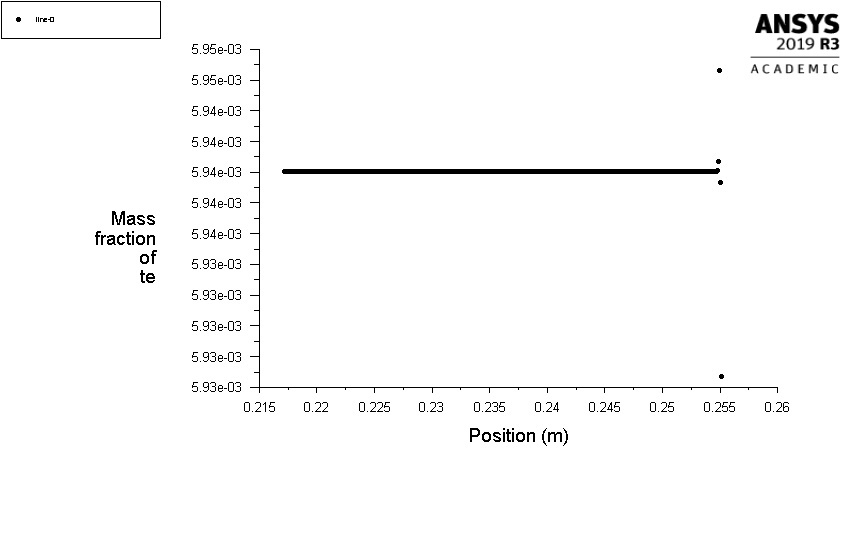But when It is auto-updated during solution, the x axis goes far beyond the scale of my geometry (my whole model is 0.3 meters long, but I have all parts in it suppressed and work only with one zone that extends between 0.217 and 0.255 m), and with every update the x-axis upper limit gets increased and gets some data poits of mass fraction=5.5 (compared to the 5.94e-3 that I prescribe in the melt as IC):nnIs this just a bug or this is an indication that I have some artifact in my problem set-up?.Thank you for your help,nnVladimirn

[Rob]

If you plot against length rather than position do you get the same result? What are you plotting on (line or mesh component)? n

[Amine Ben Hadj Ali]

1/It needs to deal with different solidus and liquidus temperature by providing the proper slope and partition coefficient. We successfully validated The modeling of heat, mass and solute transport in solidification systems V. R. VOLLER and A. D. BRENT and C. PRAKASH, Int. J. Heat Mass Transfer. Vol. 32, No. 9, pp. 1719-1731, 1989. All equations have been solved including solutal and thermal buyoancy effects.n2/You can set the mush parameter to very low value.nn

[vladr]

Rob, DrAmine,nThank you for your replies.nnRob,nThe weird plot that I was showing in the previous post was plotted on a line. When I switched to the plot of Curve Length and started running the simulation, this weird plot behavior was no longer present. nIt is worth mentioning though that I had to switch Fluent into Serial mode to do so, because when I was trying to change the plot to Curve Length it was giving me Cannot plot along curve length of line-0 error (I found the solution to this on the web- to switch into Serial).nnAll,nThe suggested solution to set Tmelt=Teutectic worked ok and seems to help with the problem of composition fluctuations. The simulation progressed up to 1/4 of the transient in 2 days (I had to use pretty fine timestep of 0.1 s to facilitate convergence), but the fluctuations are no longer present and the axial composition plot looks more like it is supposed to look. nOn the chart below the latest result (m Numerical-2) is compared to the previously discussed plot of my initial fluctuating solution and to the analytical solution that I am trying to match :n

[Rob]

Received, and passed internally. Not sure who'll respond as you're not in or my region. Bump the thread if you haven't been contacted within about a week as I think there are some holidays in the region. n

[vladr]

Rob, Surya, DrAmine,nnthank you all for your helpn

[vladr]

@Rob, I still haven't heard from anybody, please let me know If I just need to wait longer or it got stuck somewhere...nThank you

[Surya Deb]

Were you able to test the previous suggestion and were there any improvements to the result?nI would also suggest you to discuss this with your research group, specifically the analytical results from the paper. Do the analytical conditions compare exactly with the conditions of the model?nRegards,nSuryan