Learning Forum

[pnair]

Hello,

I am working on the dipole simulations on SiCO thinfilm structure. I am using box of monitors to study the far field emission patterns. I am following the theory and simulation steps in this example"https://optics.ansys.com/hc/en-us/articles/360053540493-Micro-LED" for my simulations. I have used five monitors as my thin film is on a substrate. And I have generated a plot in terms of X,Y,Z

But, I have a question related to the conversion of this plot to Angular polar plot. Is there any script to convert this plot to polar plot in terms of phi and theta? I mean how can i calculate far field plots from box of monitors using only 5 monitors?

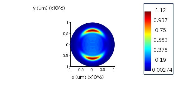
Please find the attached plot that I have generated from the above plot. And I have a question related to the X& Y axis of this plot? Do they represent the Ux and Uy direction vectors? 

 

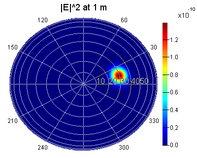
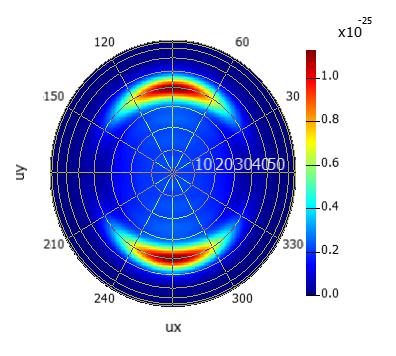
Following is the example of a farfield polar plot which I would like to generate from this:

Thankyou.

[Amrita Pati]

Hi Prabha,

I apologize for not getting back to you on your other post. I miss out on the alert emails sometimes.

The standard farfield projections are performed on a hemispherical surface but they are are flattened to be plotted in a 2D plane (the 2D plane looks like how the hemisphere would look from the top). The last plot you have shared is an example of that. But in the example link (micro-LED) you have shared, we have intentionally created an unstructured dataset to be able to plot the results on a hemisphere, as a result the plot is 3D, and x, y, and z are the direction cosines. To convert it back to 2D polar form would require a lot of co-oridnate transformation. It is not impossible, but going to be complicated especially because we don't have any exisiting scripts.

I believe the simplest approach would be to place a single monitor infront of the source, and visualize the farfield from this monitor. The monitor would plot the results in the polar form on a plane. To make sure that the single monitor collects most of the radiation you have to place the monitor close to the source, and also make the monitor as well as the simulation span large.

For example, you can plot the farfield from "z2" in your case,

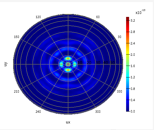
But as I said, since you will have farfield from only one monitor (we won't have the side monitors x1, x2, and y1, y2) it is important to make sure that the z2 monitor gathers most of the radiation, by making it really large. 

Regards,
Amrira

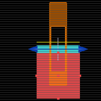
[pnair]

 

Thank you for the reply. I have a question related to the placement of a single z-normal monitor. I have placed a monitor(35x35x0.17um) exactly on the top of the structure(on the surface closer to the dipole source). I have made the simulation region larger(25x25x2um). And why I am getting different polar plots if i placed the monitor a little far from the structure surface and  far from dipole source. How did i know which plot is correct?

1) Close to the source/on the surface(blue colour thin film)

Here monitor(Z2) is placed on the top/surface of thin film.(blue layer). And I got the following polar plot.'

 

But when I place the monitor at a height/a little bit away from the surface of the sample. 

 

I got the following spectrum

So, i dont understand why I am getting two different patterns? and which one should i take as the more accurate plot?

 

[Amrita Pati]

Hi Prabha,

The differences could be because of several factors. The size of the monitor will strongly influence the result as it dictates how much of the power is collected. If there is significant radiation at the edges of the monitor, there will additional effects due to diffraction at the edges of the monitor which will also affect the farfield results. You might have to make the monitor extremely large which might end up taking a lot of time to run the simulation. The position of the monitor could also be a bit tricky and has to be addressed on a case by case basis. I also wouldn't recommend placing the monitor at/very close to the interface as some of the results would be interpolated from below the interface and some from above depending upon the exact location of the monitor in the Yee cell/mesh cell. In conclusion, both these parameters would require convergence testing to finalize their exact values.

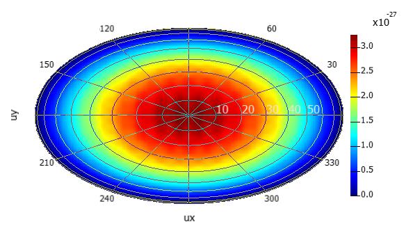
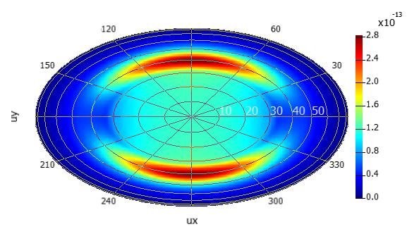
These challenges are addressed by box monitors. At the beginning, I thought it would be complicated to change the current analysis group to give the expected result. But then I realized that we could use another analysis group called "scat_ff" which can be found as "Far field from a closed box" in the Object Library. Although it says that the box is not supposed to be used with a substrate, we can delete/disable the monitor in the substrate (z1) as we are already not interested in the radiation in the -z direction in the LED example (using 5 monitors). We can set the postion and span of the "scat_ff" monitor same as the previous "farfield" analysis group. Then we can run and visualize the XY_halfspace result to look at the polar plot of the farfield:

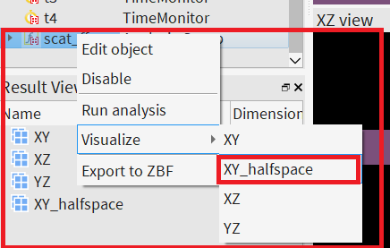
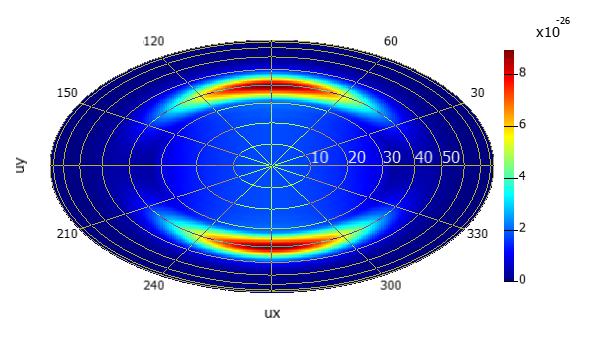
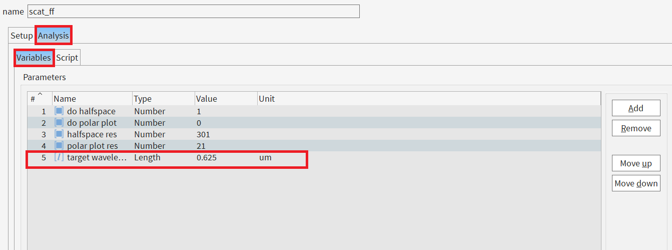
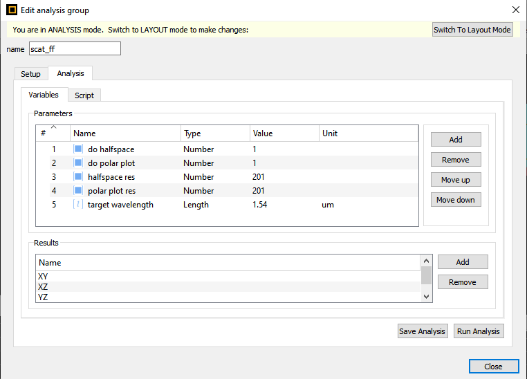
The subscripts of the XY_halfspace result indicate upper or lower halfspace. E is the field and E2 is the intensity. One thing to note here would be that unlike the previous analysis group, this one calculates the farfield for all frequency points as opposed to a single target frequency. So, if you run the analysis with the current simulation setup, it would be time consuming. I would recommend changing the dipole wavelength to a single wavelength (you could use 0.625 which is the target wavelength in the example) and then running the analysis group as a starting point to save time. I would also recommend increasing the resolution of the farfield plot by changing the corresponding parameter in the analysis group, the default resolution is rather low:

Feel free to let me know what are your thoughts.

Regards,
Amrita

[Amrita Pati]

Hi Prabha,

I was doing some testing. It turns out that we might have to make some modifications to the scat_ff analysis group. I will take look further and come back to you with more information.

Regards,
Amrita

 

[Amrita Pati]

Hi Prabha,

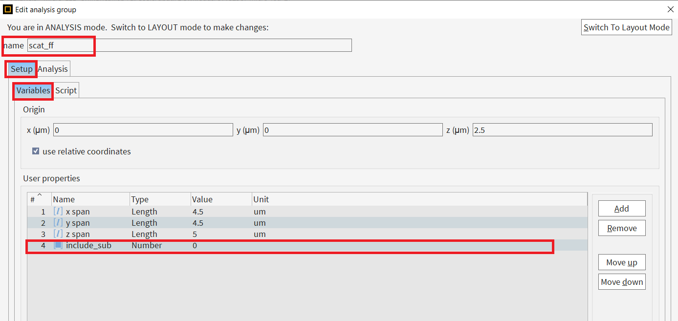
I have changed the “scat_ff” analysis group so that it can be used correctly with 5 monitors. I added a parameter called “include_sub” which lets you decide if you want to disable the monitor in the substrate. Also, added some if conditions in the Analysis script so that the if there is no substrate, we can use the symmerty conditions depending upon whether or not required. But if it is include_sub is false, the monitor data from “z1” is completely ignored. Before making these changes, even if you disable the monitor, it would consider symmetry conditions and manipulate the values of z1, to get the values of z2. I can not share the files with you directly as ALF doesn’t permit it. But here are the screenshots and code snippets:

 

1. First add “scat_ff” from the Object Library (Far field from a closed box).
2. Change it’s span and position (make it same as the previous farfield group).
3. Edit it, go to “Setup–>Variables“, add a property called "include_sub" of type Number:
   
   
4. Go to Setup–>Script, replace the existing code by the following:

##############################################
# Far field from closed box
# This script sets up the monitor box
#
# Input properties
# x,y,z span: span of the box of monitors
#
# Tags: far field projection closed box
#
# Copyright 2012 Lumerical Solutions Inc
##############################################
# simplify variable names by removing spaces
x_span = %x span%;
y_span = %y span%;
z_span = %z span%;

select(“z1”);
set(“x”,0);
set(“x span”,x_span);
set(“y”,0);
set(“y span”,y_span);
set(“z”,-z_span/2);
set(“enabled”,include_sub);

select(“z2”);
set(“x”,0);
set(“x span”,x_span);
set(“y”,0);
set(“y span”,y_span);
set(“z”,z_span/2);

select(“x1”);
set(“x”,-x_span/2);
set(“y”,0);
set(“y span”,y_span);
set(“z”,0);
set(“z span”,z_span);

select(“x2”);
set(“x”,x_span/2);
set(“y”,0);
set(“y span”,y_span);
set(“z”,0);
set(“z span”,z_span);

select(“y1”);
set(“x”,0);
set(“x span”,x_span);
set(“y”,-y_span/2);
set(“z”,0);
set(“z span”,z_span);

select(“y2”);
set(“x”,0);
set(“x span”,x_span);
set(“y”,y_span/2);
set(“z”,0);
set(“z span”,z_span);

select(“index”);
set(“x”,x_span/2);
set(“y”,y_span/2);
set(“z”,0);
set(“x span”,0);
set(“y span”,0);
set(“z span”,0);

5. Go to Analysis–>Script, replace the existing code by the following:

##############################################

# Far field from closed box

# This script calculates scattering cross-section and far field projection in half space

#

# Note: The far field projection calculation assumes that all of the monitors

# are in a single homogeneous material (i.e. there is no substrate)

# If a substrate is present, results from this object will be invalid.

# If multiple frequency points are collected, the projection can be slow!! One could reduce the halfspace resolution for faster analysis.

# For more information, see http://docs.lumerical.com/en/layout_analysis_projections_from_monitor.html

#

# symm x,y,z: symmetry boundary conditions

# 0 for no symmetry, 1 for symmetric, -1 for antisymmetric

# Autodetection is managed by examining fields at the symmetry boundary

# For more information, see http://docs.lumerical.com/en/index.html?ref_sim_obj_symmetric_anti-symmetric.html

#

# do halfspace: Calculate the far field in the full half space for all frequencies. This takes longer than the 1D radar line cross sections. 1 for yes, 0 for no

# do polar plot: Calculate the far field scattering angular distribution for a specified target wavelength. 1 for yes, 0 for no

# target wavelength: Desired wavelength for polar plot. The closest wavelength recorded by the monitors will be found and used for the plot.

# halfspace res: Define the resolution of the half space projection. This will significantly affect the time to run the analysis.

# polar plot res: Define the resolution of the polat plots.

#

# Output properties

# XY, YZ, XZ: E, |E|^2, |H|^2 far field profile of scattered field in plane, as a function of frequency

# XY_halfspace: E, |E|^2, |H|^2 in full upper/lower half space,, as a function of frequency. Similar to standard projection from a single monitor

#

# Tags: far field projection closed box

#

# Copyright 2015 Lumerical Solutions Inc

##############################################



##############################################

# automatically unfold field data if symmetry BC is applied

if (havedata(“x1”, “f”)) {

symm_x = 0;

} else {

xtemp = getdata(“y2”, “x”);

ztemp = getdata(“y2”, “z”);

Eztemp = pinch(getdata(“y2”, “Ez”));



Ez2mid = sum(Eztemp(round(length(xtemp)/2), 1:length(ztemp))^2);

if (Ez2mid != 0) {

symm_x = 1;

} else {

symm_x = -1;

}

}



if (havedata(“y1”, “f”)) {

symm_y = 0;

} else {

ytemp = getdata(“x2”, “y”);

ztemp = getdata(“x2”, “z”);

Eztemp = pinch(getdata(“x2”, “Ez”));



Ez2mid = sum(Eztemp(round(length(ytemp)/2), 1:length(ztemp))^2);

if (Ez2mid != 0) {

symm_y = 1;

} else {

symm_y = -1;

}

}

if(include_sub){

if (havedata(“z1”, “f”)) {

symm_z = 0;

} else {

xtemp = getdata(“y2”, “x”);

ztemp = getdata(“y2”, “z”);

Eytemp = pinch(getdata(“y2”, “Ey”));



Ey2mid = sum(Eytemp(1:length(xtemp), round(length(ztemp)/2))^2);

if (Ey2mid != 0) {

symm_z = 1;

} else {

symm_z = -1;

}

}

}

f = getdata(“x2″,”f”); # get freqency data



if (havedata(“index”,”index_x”)) { # get refractive index. Required to calcualte H2 from E2

n_index = getdata(“index”,”index_x”);

} else {

n_index = getdata(“index”,”index_z”);

}

##############################################





# define the angular resolution

phi = linspace(0,360,%polar plot res%); # user-modifiable in the Variables tab

npts = length(phi);



# define the field data matrices for angular distribution

E_xy = matrix(npts, 3, length(f)); # 3 for x, y, z component

E_yz = matrix(npts, 3, length(f)); # 3 for x, y, z component

E_xz = matrix(npts, 3, length(f)); # 3 for x, y, z component

E2_xy = matrix(npts,length(f));

E2_yz = matrix(npts,length(f));

E2_xz = matrix(npts,length(f));

H2_xy = matrix(npts,length(f));

H2_yz = matrix(npts,length(f));

H2_xz = matrix(npts,length(f));





# Identify the closest wavelength to target:

target_wavelength = %target wavelength%;

i_target = find(f,c/target_wavelength);

?”Target wavelength = ” + num2str(target_wavelength);

?”Wavelength used = ” + num2str(c/f(i_target));





if (havedata(“z2″,”Ex”)) { # have z data, 3D simulation



##############################################

# Angular distribution calculation for a 3D simulation begins



for (i = 1:length(f)){ # loop for all frequencies



# print the frequency point number running in the loop

?”Angular distribution i=”+num2str(i)+”, “+num2str(c/f(i)*1e6)+”um”;



n = n_index(i); # select the frequency point for the index



######## x-y plane (phi=0 corresponds to the direction (1,0,0))

?” Projecting in x-y plane”;

x = cos(phi*pi/180); y = sin(phi*pi/180); z = 0;



# Calculate far field by summing contribution from each monitor

temp = farfieldexact(“x2”,x,y,z,i) + farfieldexact(“y2”,x,y,z,i) + farfieldexact(“z2″,x,y,z,i);

if(havedata(“x1″)){

temp = temp – farfieldexact(“x1″,x,y,z,i);

}else{

temp2 = farfieldexact(“x2″,-x,y,z,i);

s = symm_x*[1,-1,-1];

temp2(1:npts,1) = s(1)*temp2(1:npts,1);

temp2(1:npts,2) = s(2)*temp2(1:npts,2);

temp2(1:npts,3) = s(3)*temp2(1:npts,3);

temp = temp – temp2;

}

if(havedata(“y1″)){

temp = temp – farfieldexact(“y1″,x,y,z,i);

}else{

temp2 = farfieldexact(“y2″,x,-y,z,i);

s = symm_y*[-1,1,-1];

temp2(1:npts,1) = s(1)*temp2(1:npts,1);

temp2(1:npts,2) = s(2)*temp2(1:npts,2);

temp2(1:npts,3) = s(3)*temp2(1:npts,3);

temp = temp – temp2;

}

if(include_sub){

if(havedata(“z1″)){

temp = temp – farfieldexact(“z1″,x,y,z,i);

}else{

temp2 = farfieldexact(“z2″,x,y,-z,i);

s = symm_z*[-1,-1,1];

temp2(1:npts,1) = s(1)*temp2(1:npts,1);

temp2(1:npts,2) = s(2)*temp2(1:npts,2);

temp2(1:npts,3) = s(3)*temp2(1:npts,3);

temp = temp – temp2;

}

}

E_xy (1:length(phi), 1:3, i) = temp;

E2_xy (1:length(phi), i) = sum(abs(temp)^2,2); # E2 = |Ex|^2 + |Ey|^2 + |Ez|^2

H2_xy (1:length(phi), i) = E2_xy (1:length(phi), i) * n^2 * eps0/mu0; # for a plane wave, E^2 and H^2 only differ by a factor of n^2*eps0/mu0







######## y-z plane (phi=0 corresponds to the direction (0,1,0))

?” Projecting in y-z plane”;

x = 0; y = cos(phi*pi/180); z = sin(phi*pi/180);



# Calculate far field by summing contribution from each monitor

temp = farfieldexact(“x2”,x,y,z,i) + farfieldexact(“y2”,x,y,z,i) + farfieldexact(“z2″,x,y,z,i);

if(havedata(“x1″)){

temp = temp – farfieldexact(“x1″,x,y,z,i);

}else{

temp2 = farfieldexact(“x2″,-x,y,z,i);

s = symm_x*[1,-1,-1];

temp2(1:npts,1) = s(1)*temp2(1:npts,1);

temp2(1:npts,2) = s(2)*temp2(1:npts,2);

temp2(1:npts,3) = s(3)*temp2(1:npts,3);

temp = temp – temp2;

}

if(havedata(“y1″)){

temp = temp – farfieldexact(“y1″,x,y,z,i);

}else{

temp2 = farfieldexact(“y2″,x,-y,z,i);

s = symm_y*[-1,1,-1];

temp2(1:npts,1) = s(1)*temp2(1:npts,1);

temp2(1:npts,2) = s(2)*temp2(1:npts,2);

temp2(1:npts,3) = s(3)*temp2(1:npts,3);

temp = temp – temp2;

}

if(include_sub){

if(havedata(“z1″)){

temp = temp – farfieldexact(“z1″,x,y,z,i);

}else{

temp2 = farfieldexact(“z2″,x,y,-z,i);

s = symm_z*[-1,-1,1];

temp2(1:npts,1) = s(1)*temp2(1:npts,1);

temp2(1:npts,2) = s(2)*temp2(1:npts,2);

temp2(1:npts,3) = s(3)*temp2(1:npts,3);

temp = temp – temp2;

}

}

E_yz (1:length(phi), 1:3, i) = temp;

E2_yz (1:length(phi), i) = sum(abs(temp)^2,2); # E2 = |Ex|^2 + |Ey|^2 + |Ez|^2

H2_yz (1:length(phi), i) = E2_yz (1:length(phi), i) * n^2 * eps0/mu0; # for a plane wave, E^2 and H^2 only differ by a factor of n^2*eps0/mu0







######### x-z plane (phi=0 corresponds to the direction (1,0,0))

?” Projecting in x-z plane”;

x = cos(phi*pi/180); y = 0; z = sin(phi*pi/180);



# Calculate far field by summing contribution from each monitor

temp = farfieldexact(“x2”,x,y,z,i) + farfieldexact(“y2”,x,y,z,i) + farfieldexact(“z2″,x,y,z,i);

if(havedata(“x1″)){

temp = temp – farfieldexact(“x1″,x,y,z,i);

}else{

temp2 = farfieldexact(“x2″,-x,y,z,i);

s = symm_x*[1,-1,-1];

temp2(1:npts,1) = s(1)*temp2(1:npts,1);

temp2(1:npts,2) = s(2)*temp2(1:npts,2);

temp2(1:npts,3) = s(3)*temp2(1:npts,3);

temp = temp – temp2;

}

if(havedata(“y1″)){

temp = temp – farfieldexact(“y1″,x,y,z,i);

}else{

temp2 = farfieldexact(“y2″,x,-y,z,i);

s = symm_y*[-1,1,-1];

temp2(1:npts,1) = s(1)*temp2(1:npts,1);

temp2(1:npts,2) = s(2)*temp2(1:npts,2);

temp2(1:npts,3) = s(3)*temp2(1:npts,3);

temp = temp – temp2;

}

if(include_sub){

if(havedata(“z1″)){

temp = temp – farfieldexact(“z1″,x,y,z,i);

}else{

temp2 = farfieldexact(“z2″,x,y,-z,i);

s = symm_z*[-1,-1,1];

temp2(1:npts,1) = s(1)*temp2(1:npts,1);

temp2(1:npts,2) = s(2)*temp2(1:npts,2);

temp2(1:npts,3) = s(3)*temp2(1:npts,3);

temp = temp – temp2;

}

}

E_xz (1:length(phi), 1:3, i) = temp;

E2_xz (1:length(phi), i) = sum(abs(temp)^2,2); # E2 = |Ex|^2 + |Ey|^2 + |Ez|^2

H2_xz (1:length(phi), i) = E2_xz (1:length(phi), i) * n^2 * eps0/mu0; # for a plane wave, E^2 and H^2 only differ by a factor of n^2*eps0/mu0



} # end of the angular distribution for loop



if (%do polar plot%) { # polar plot for target wavelength

polar(phi*pi/180, E2_xy(1:length(phi), i_target), E2_yz(1:length(phi), i_target), E2_xz(1:length(phi), i_target),

”angle (degrees)”, “|E|^2”, “|E|^2 vs angle @ “+num2str(c/f(i_target)*1e6)+”um”);

legend(“xy plane”,”yz plane”,”xz plane”);

} # end of if polar plot



# create datasets for XY, YZ, XZ for angular distribution

XY = matrixdataset(“XY”);

XY.addparameter(“phi”,phi*pi/180.); #phi angle in radians

XY.addparameter(“lambda”,c/f,”f”,f);

XY.addattribute(“E”,pinch(E_xy,2,1),pinch(E_xy,2,2),pinch(E_xy,2,3)); # Ex, Ey, Ez

XY.addattribute(“E2″,E2_xy);

XY.addattribute(“H2″,H2_xy);



YZ = matrixdataset(“YZ”);

YZ.addparameter(“phi”,phi*pi/180.); #phi angle in radians

YZ.addparameter(“lambda”,c/f,”f”,f);

YZ.addattribute(“E”,pinch(E_yz,2,1),pinch(E_yz,2,2),pinch(E_yz,2,3)); # Ex, Ey, Ez

YZ.addattribute(“E2″,E2_yz);

YZ.addattribute(“H2″,H2_yz);



XZ = matrixdataset(“XZ”);

XZ.addparameter(“phi”,phi*pi/180.); #phi angle in radians

XZ.addparameter(“lambda”,c/f,”f”,f);

XZ.addattribute(“E”,pinch(E_xz,2,1),pinch(E_xz,2,2),pinch(E_xz,2,3)); # Ex, Ey, Ez

XZ.addattribute(“E2″,E2_xz);

XZ.addattribute(“H2″,H2_xz);

# end of the angular distribution for a 3D simulation

##############################################



##############################################

# Halfspace calculation for a 3D simulation begins



# calculate the far field in XY upper/lower half space

if (%do halfspace%) {



res = %halfspace res%; # projection resolution, user-modifiable in the Variables tab

u1 = linspace(-1,1,res);

u2 = u1;

X = meshgridx(u1,u2); # These three lines define the orientation of the hemisphere (ie. XY based halfspace)

Y = meshgridy(u1,u2);

Z = sqrt(1-X^2-Y^2);

filter = abs(imag(Z))<=0; # filter out any values outside of hemisphere

filter2=matrix(res,res,length(f)); # same as filter, just for all frequencies

filter3=matrix(res,res,3,length(f)); # same as filter2, just for all frequencies, Ex, Ey, Ez

for (j=1:length(f)){ # just for filter2 and fitler3 for all frequencies

filter2(1:res,1:res,j)=filter;

filter3(1:res,1:res,1,j)=filter; filter3(1:res,1:res,2,j)=filter; filter3(1:res,1:res,3,j)=filter;

}

x = reshape(X,[res^2,1]); # reshape coordinate matrix into a vector. This is the required form for farfieldexact.

y = reshape(Y,[res^2,1]);

z = reshape(Z,[res^2,1]);

x = [x,x]; # Concatenate a 2nd copy of the vector, for the lower half space

y = [y,y];

z = [z,-z];

npts = length(z); # size of position vector



# define halfspace dataset

E_XY_halfspace = matrix (2*res^2,3,length(f));

E2_XY_halfspace = matrix (2*res^2,length(f));

H2_XY_halfspace = matrix (2*res^2,length(f));





for (i = 1 : length(f)) { # loop for all frequency points



?”Projecting in XY upper half space, i=” + num2str(i)+”, “+num2str(c/f(i)*1e6)+”um”;

# Calculate far field by summing contribution from each monitor

temp = farfieldexact(“x2”,x,y,z,i) + farfieldexact(“y2”,x,y,z,i) + farfieldexact(“z2″,x,y,z,i);

if(havedata(“x1″)){

temp = temp – farfieldexact(“x1″,x,y,z,i);

}else{

temp2 = farfieldexact(“x2″,-x,y,z,i);

s = symm_x*[1,-1,-1];

temp2(1:npts,1) = s(1)*temp2(1:npts,1);

temp2(1:npts,2) = s(2)*temp2(1:npts,2);

temp2(1:npts,3) = s(3)*temp2(1:npts,3);

temp = temp – temp2;

}

if(havedata(“y1″)){

temp = temp – farfieldexact(“y1″,x,y,z,i);

}else{

temp2 = farfieldexact(“y2″,x,-y,z,i);

s = symm_y*[-1,1,-1];

temp2(1:npts,1) = s(1)*temp2(1:npts,1);

temp2(1:npts,2) = s(2)*temp2(1:npts,2);

temp2(1:npts,3) = s(3)*temp2(1:npts,3);

temp = temp – temp2;

}

if(include_sub){

if(havedata(“z1″)){

temp = temp – farfieldexact(“z1″,x,y,z,i);

}else{

temp2 = farfieldexact(“z2″,x,y,-z,i);

s = symm_z*[-1,-1,1];

temp2(1:npts,1) = s(1)*temp2(1:npts,1);

temp2(1:npts,2) = s(2)*temp2(1:npts,2);

temp2(1:npts,3) = s(3)*temp2(1:npts,3);

temp = temp – temp2;

}

}



E_XY_halfspace (1:2*res^2,1:3,i) = temp;

E2_XY_halfspace (1:2*res^2,i)= sum(abs(temp)^2,2); # E2 = |Ex|^2 + |Ey|^2 + |Ez|^2

} # end of halfspace for loop



E_XY_upper_halfspace = E_XY_halfspace(1:res^2,1:3,1:length(f)); # separate the upper/lower data

E_XY_lower_halfspace = E_XY_halfspace((res^2+1):(2*res^2),1:3,1:length(f));

E_XY_upper_halfspace = reshape(E_XY_upper_halfspace,[res,res,3,length(f)]); # reshape the data back into a 2D matrix

E_XY_lower_halfspace = reshape(E_XY_lower_halfspace,[res,res,3,length(f)]);

E_XY_upper_halfspace = E_XY_upper_halfspace*filter3; # set all values outside of hemisphere (ie. the corners of the matrices) to zero

E_XY_lower_halfspace = E_XY_lower_halfspace*filter3;



E2_XY_upper_halfspace = E2_XY_halfspace(1:res^2,1:length(f)); # separate the upper/lower data

E2_XY_lower_halfspace = E2_XY_halfspace((res^2+1):(2*res^2),1:length(f));

E2_XY_upper_halfspace = reshape(E2_XY_upper_halfspace,[res,res,length(f)]); # reshape the data back into a 2D matrix

E2_XY_lower_halfspace = reshape(E2_XY_lower_halfspace,[res,res,length(f)]);

E2_XY_upper_halfspace = E2_XY_upper_halfspace*filter2; # set all values outside of hemisphere (ie. the corners of the matrices) to zero

E2_XY_lower_halfspace = E2_XY_lower_halfspace*filter2;



# create halfspace dataset

XY_halfspace = matrixdataset(“XY_halfspace”);

XY_halfspace.addparameter(“ux”,u1);

XY_halfspace.addparameter(“uy”,u2);

XY_halfspace.addparameter(“lambda”,c/f,”f”,f);

XY_halfspace.addattribute(“E_upper”,pinch(E_XY_upper_halfspace,3,1),pinch(E_XY_upper_halfspace,3,2),pinch(E_XY_upper_halfspace,3,3));

XY_halfspace.addattribute(“E_lower”,pinch(E_XY_lower_halfspace,3,1),pinch(E_XY_lower_halfspace,3,2),pinch(E_XY_lower_halfspace,3,3));

XY_halfspace.addattribute(“E2_upper”,E2_XY_upper_halfspace);

XY_halfspace.addattribute(“E2_lower”,E2_XY_lower_halfspace);

XY_halfspace.addattribute(“H2_upper”,E2_XY_upper_halfspace * n^2*eps0/mu0);

XY_halfspace.addattribute(“H2_lower”,E2_XY_lower_halfspace * n^2*eps0/mu0);

}

# end of the halfspace calculation for a 3D simulation

##############################################



# end of 3D



} else {

##############################################

# Angular distribution for a 2D simulation, only for the XY plane
for (i = 1 : length(f)) { # for all frequency points
n = n_index(i); # select the frequency point for the index

# x-y plane (phi=0 corresponds to the direction (0,1,0))
?” Projecting in x-y plane. 2D simulation.”;

x = -sin(phi*pi/180);
y = cos(phi*pi/180);
z = 0;

temp = farfieldexact(“x2”,x,y,i) + farfieldexact(“y2″,x,y,i);
if(havedata(“x1″)){
temp = temp – farfieldexact(“x1″,x,y,i);
}else{
temp2 = farfieldexact(“x2″,-x,y,i);
s = symm_x*[1,-1,-1];
temp2(1:length(phi),1) = s(1)*temp2(1:length(phi),1);
temp2(1:length(phi),2) = s(2)*temp2(1:length(phi),2);
temp2(1:length(phi),3) = s(3)*temp2(1:length(phi),3);
temp = temp – temp2;
}
if(havedata(“y1″)){
temp = temp – farfieldexact(“y1″,x,y,i);
}else{
temp2 = farfieldexact(“y2″,x,-y,i);
s = symm_y*[-1,1,-1];
temp2(1:length(phi),1) = s(1)*temp2(1:length(phi),1);
temp2(1:length(phi),2) = s(2)*temp2(1:length(phi),2);
temp2(1:length(phi),3) = s(3)*temp2(1:length(phi),3);
temp = temp – temp2;
}

E_xy (1:length(phi), 1:3, i) = temp;
E2_xy (1:length(phi), i) = sum(abs(temp)^2,2); # E2 = |Ex|^2 + |Ey|^2 + |Ez|^2
H2_xy (1:length(phi), i) = E2_xy (1:length(phi), i) * n^2 * eps0/mu0; # for a plane wave, E^2 and H^2 only differ by a factor of n^2*eps0/mu0

} # end of for loop 2D

if (%do polar plot%) { # polar plot for target wavelength
polar(phi*pi/180, E2_xy(1:length(phi), i_target), “angle (degrees)”, “|E|^2”, “|E|^2 vs angle @ “+num2str(c/f(i_target)*1e6)+”um”);
legend(“xy plane”);
} # end of if polar plot

# create dataset for XY
XY = matrixdataset(“XY”);
XY.addparameter(“phi”,phi*pi/180.); #phi angle in radians
XY.addparameter(“lambda”,c/f,”f”,f);
XY.addattribute(“E”,pinch(E_xy,2,1),pinch(E_xy,2,2),pinch(E_xy,2,3)); # Ex, Ey, Ez
XY.addattribute(“E2″,E2_xy);
XY.addattribute(“H2″,H2_xy);
} # end of angular distribution for 2D simulation
########################################

6. Contrary to one of the points I previously made, you can perform a broadband simulation and perform the farfield projection over a single target wavelength:

Feel free to let me know if you have any questions.

Regards,
Amrita

 

[pnair]

Hello Amrita,

Thank you for the reply and a detailed explanation of farfield analysis group and the corrected script.

I run the simulation with the script suggested here. But, It is generating an error:

Target wavelength = 1.54e-06

Wavelength used = 1.54e-06

Angular distribution i=1, 1.54um

Projecting in x-y plane

Projecting in y-z plane

Projecting in x-z plane

Error: Result XY_halfspace: variable not found.

And, I am not able to visualize the farfied data in the xy_half space and its showing"failed to calculate results"

Please find the attached script that you have suggested here and I have used the same script for the simulations:

##############################################

# Far field from closed box

# This script calculates scattering cross-section and far field projection in half space

#

# Note: The far field projection calculation assumes that all of the monitors

# are in a single homogeneous material (i.e. there is no substrate)

# If a substrate is present, results from this object will be invalid.

# If multiple frequency points are collected, the projection can be slow!! One could reduce the halfspace resolution for faster analysis.

# For more information, see http://docs.lumerical.com/en/layout_analysis_projections_from_monitor.html

#

# symm x,y,z: symmetry boundary conditions

# 0 for no symmetry, 1 for symmetric, -1 for antisymmetric

# Autodetection is managed by examining fields at the symmetry boundary

# For more information, see http://docs.lumerical.com/en/index.html?ref_sim_obj_symmetric_anti-symmetric.html

#

# do halfspace: Calculate the far field in the full half space for all frequencies. This takes longer than the 1D radar line cross sections. 1 for yes, 0 for no

# do polar plot: Calculate the far field scattering angular distribution for a specified target wavelength. 1 for yes, 0 for no

# target wavelength: Desired wavelength for polar plot. The closest wavelength recorded by the monitors will be found and used for the plot.

# halfspace res: Define the resolution of the half space projection. This will significantly affect the time to run the analysis.

# polar plot res: Define the resolution of the polat plots.

#

# Output properties

# XY, YZ, XZ: E, |E|^2, |H|^2 far field profile of scattered field in plane, as a function of frequency

# XY_halfspace: E, |E|^2, |H|^2 in full upper/lower half space,, as a function of frequency. Similar to standard projection from a single monitor

#

# Tags: far field projection closed box

#

# Copyright 2015 Lumerical Solutions Inc

##############################################

 

##############################################

# automatically unfold field data if symmetry BC is applied

if (havedata("x1", "f")) {

symm_x = 0;

} else {

xtemp = getdata("y2", "x");

ztemp = getdata("y2", "z");

Eztemp = pinch(getdata("y2", "Ez"));

 

Ez2mid = sum(Eztemp(round(length(xtemp)/2), 1:length(ztemp))^2);

if (Ez2mid != 0) {

symm_x = 1;

} else {

symm_x = -1;

}

}

 

if (havedata("y1", "f")) {

symm_y = 0;

} else {

ytemp = getdata("x2", "y");

ztemp = getdata("x2", "z");

Eztemp = pinch(getdata("x2", "Ez"));

 

Ez2mid = sum(Eztemp(round(length(ytemp)/2), 1:length(ztemp))^2);

if (Ez2mid != 0) {

symm_y = 1;

} else {

symm_y = -1;

}

}

 

if(include_sub){

if (havedata("z1", "f")) {

symm_z = 0;

} else {

xtemp = getdata("y2", "x");

ztemp = getdata("y2", "z");

Eytemp = pinch(getdata("y2", "Ey"));

 

Ey2mid = sum(Eytemp(1:length(xtemp), round(length(ztemp)/2))^2);

if (Ey2mid != 0) {

symm_z = 1;

} else {

symm_z = -1;

}

}

}

f = getdata("x2","f"); # get freqency data

 

if (havedata("index","index_x")) { # get refractive index. Required to calcualte H2 from E2

n_index = getdata("index","index_x");

} else {

n_index = getdata("index","index_z");

}

##############################################

 

 

# define the angular resolution

phi = linspace(0,360,%polar plot res%); # user-modifiable in the Variables tab

npts = length(phi);

 

# define the field data matrices for angular distribution

E_xy = matrix(npts, 3, length(f)); # 3 for x, y, z component

E_yz = matrix(npts, 3, length(f)); # 3 for x, y, z component

E_xz = matrix(npts, 3, length(f)); # 3 for x, y, z component

E2_xy = matrix(npts,length(f));

E2_yz = matrix(npts,length(f));

E2_xz = matrix(npts,length(f));

H2_xy = matrix(npts,length(f));

H2_yz = matrix(npts,length(f));

H2_xz = matrix(npts,length(f));

 

 

# Identify the closest wavelength to target:

target_wavelength = %target wavelength%;

i_target = find(f,c/target_wavelength);

?"Target wavelength = " + num2str(target_wavelength);

?"Wavelength used = " + num2str(c/f(i_target));

 

 

if (havedata("z2","Ex")) { # have z data, 3D simulation

 

##############################################

# Angular distribution calculation for a 3D simulation begins

 

for (i = 1:length(f)){ # loop for all frequencies

 

# print the frequency point number running in the loop

?"Angular distribution i="+num2str(i)+", "+num2str(c/f(i)*1e6)+"um";

 

n = n_index(i); # select the frequency point for the index

 

######## x-y plane (phi=0 corresponds to the direction (1,0,0))

?" Projecting in x-y plane";

x = cos(phi*pi/180); y = sin(phi*pi/180); z = 0;

 

# Calculate far field by summing contribution from each monitor

temp = farfieldexact("x2",x,y,z,i) + farfieldexact("y2",x,y,z,i) + farfieldexact("z2",x,y,z,i);

if(havedata("x1")){

temp = temp - farfieldexact("x1",x,y,z,i);

}else{

temp2 = farfieldexact("x2",-x,y,z,i);

s = symm_x*[1,-1,-1];

temp2(1:npts,1) = s(1)*temp2(1:npts,1);

temp2(1:npts,2) = s(2)*temp2(1:npts,2);

temp2(1:npts,3) = s(3)*temp2(1:npts,3);

temp = temp - temp2;

}

if(havedata("y1")){

temp = temp - farfieldexact("y1",x,y,z,i);

}else{

temp2 = farfieldexact("y2",x,-y,z,i);

s = symm_y*[-1,1,-1];

temp2(1:npts,1) = s(1)*temp2(1:npts,1);

temp2(1:npts,2) = s(2)*temp2(1:npts,2);

temp2(1:npts,3) = s(3)*temp2(1:npts,3);

temp = temp - temp2;

}

if(include_sub){

if(havedata("z1")){

temp = temp - farfieldexact("z1",x,y,z,i);

}else{

temp2 = farfieldexact("z2",x,y,-z,i);

s = symm_z*[-1,-1,1];

temp2(1:npts,1) = s(1)*temp2(1:npts,1);

temp2(1:npts,2) = s(2)*temp2(1:npts,2);

temp2(1:npts,3) = s(3)*temp2(1:npts,3);

temp = temp - temp2;

}

}

E_xy (1:length(phi), 1:3, i) = temp;

E2_xy (1:length(phi), i) = sum(abs(temp)^2,2); # E2 = |Ex|^2 + |Ey|^2 + |Ez|^2

H2_xy (1:length(phi), i) = E2_xy (1:length(phi), i) * n^2 * eps0/mu0; # for a plane wave, E^2 and H^2 only differ by a factor of n^2*eps0/mu0

 

 

 

######## y-z plane (phi=0 corresponds to the direction (0,1,0))

?" Projecting in y-z plane";

x = 0; y = cos(phi*pi/180); z = sin(phi*pi/180);

 

# Calculate far field by summing contribution from each monitor

temp = farfieldexact("x2",x,y,z,i) + farfieldexact("y2",x,y,z,i) + farfieldexact("z2",x,y,z,i);

if(havedata("x1")){

temp = temp - farfieldexact("x1",x,y,z,i);

}else{

temp2 = farfieldexact("x2",-x,y,z,i);

s = symm_x*[1,-1,-1];

temp2(1:npts,1) = s(1)*temp2(1:npts,1);

temp2(1:npts,2) = s(2)*temp2(1:npts,2);

temp2(1:npts,3) = s(3)*temp2(1:npts,3);

temp = temp - temp2;

}

if(havedata("y1")){

temp = temp - farfieldexact("y1",x,y,z,i);

}else{

temp2 = farfieldexact("y2",x,-y,z,i);

s = symm_y*[-1,1,-1];

temp2(1:npts,1) = s(1)*temp2(1:npts,1);

temp2(1:npts,2) = s(2)*temp2(1:npts,2);

temp2(1:npts,3) = s(3)*temp2(1:npts,3);

temp = temp - temp2;

}

if(include_sub){

if(havedata("z1")){

temp = temp - farfieldexact("z1",x,y,z,i);

}else{

temp2 = farfieldexact("z2",x,y,-z,i);

s = symm_z*[-1,-1,1];

temp2(1:npts,1) = s(1)*temp2(1:npts,1);

temp2(1:npts,2) = s(2)*temp2(1:npts,2);

temp2(1:npts,3) = s(3)*temp2(1:npts,3);

temp = temp - temp2;

}

}

E_yz (1:length(phi), 1:3, i) = temp;

E2_yz (1:length(phi), i) = sum(abs(temp)^2,2); # E2 = |Ex|^2 + |Ey|^2 + |Ez|^2

H2_yz (1:length(phi), i) = E2_yz (1:length(phi), i) * n^2 * eps0/mu0; # for a plane wave, E^2 and H^2 only differ by a factor of n^2*eps0/mu0

 

 

 

######### x-z plane (phi=0 corresponds to the direction (1,0,0))

?" Projecting in x-z plane";

x = cos(phi*pi/180); y = 0; z = sin(phi*pi/180);

 

# Calculate far field by summing contribution from each monitor

temp = farfieldexact("x2",x,y,z,i) + farfieldexact("y2",x,y,z,i) + farfieldexact("z2",x,y,z,i);

if(havedata("x1")){

temp = temp - farfieldexact("x1",x,y,z,i);

}else{

temp2 = farfieldexact("x2",-x,y,z,i);

s = symm_x*[1,-1,-1];

temp2(1:npts,1) = s(1)*temp2(1:npts,1);

temp2(1:npts,2) = s(2)*temp2(1:npts,2);

temp2(1:npts,3) = s(3)*temp2(1:npts,3);

temp = temp - temp2;

}

if(havedata("y1")){

temp = temp - farfieldexact("y1",x,y,z,i);

}else{

temp2 = farfieldexact("y2",x,-y,z,i);

s = symm_y*[-1,1,-1];

temp2(1:npts,1) = s(1)*temp2(1:npts,1);

temp2(1:npts,2) = s(2)*temp2(1:npts,2);

temp2(1:npts,3) = s(3)*temp2(1:npts,3);

temp = temp - temp2;

}

if(include_sub){

if(havedata("z1")){

temp = temp - farfieldexact("z1",x,y,z,i);

}else{

temp2 = farfieldexact("z2",x,y,-z,i);

s = symm_z*[-1,-1,1];

temp2(1:npts,1) = s(1)*temp2(1:npts,1);

temp2(1:npts,2) = s(2)*temp2(1:npts,2);

temp2(1:npts,3) = s(3)*temp2(1:npts,3);

temp = temp - temp2;

}

}

E_xz (1:length(phi), 1:3, i) = temp;

E2_xz (1:length(phi), i) = sum(abs(temp)^2,2); # E2 = |Ex|^2 + |Ey|^2 + |Ez|^2

H2_xz (1:length(phi), i) = E2_xz (1:length(phi), i) * n^2 * eps0/mu0; # for a plane wave, E^2 and H^2 only differ by a factor of n^2*eps0/mu0

 

} # end of the angular distribution for loop

 

if (%do polar plot%) { # polar plot for target wavelength

polar(phi*pi/180, E2_xy(1:length(phi), i_target), E2_yz(1:length(phi), i_target), E2_xz(1:length(phi), i_target),

"angle (degrees)", "|E|^2", "|E|^2 vs angle @ "+num2str(c/f(i_target)*1e6)+"um");

legend("xy plane","yz plane","xz plane");

} # end of if polar plot

 

# create datasets for XY, YZ, XZ for angular distribution

XY = matrixdataset("XY");

XY.addparameter("phi",phi*pi/180.); #phi angle in radians

XY.addparameter("lambda",c/f,"f",f);

XY.addattribute("E",pinch(E_xy,2,1),pinch(E_xy,2,2),pinch(E_xy,2,3)); # Ex, Ey, Ez

XY.addattribute("E2",E2_xy);

XY.addattribute("H2",H2_xy);

 

YZ = matrixdataset("YZ");

YZ.addparameter("phi",phi*pi/180.); #phi angle in radians

YZ.addparameter("lambda",c/f,"f",f);

YZ.addattribute("E",pinch(E_yz,2,1),pinch(E_yz,2,2),pinch(E_yz,2,3)); # Ex, Ey, Ez

YZ.addattribute("E2",E2_yz);

YZ.addattribute("H2",H2_yz);

 

XZ = matrixdataset("XZ");

XZ.addparameter("phi",phi*pi/180.); #phi angle in radians

XZ.addparameter("lambda",c/f,"f",f);

XZ.addattribute("E",pinch(E_xz,2,1),pinch(E_xz,2,2),pinch(E_xz,2,3)); # Ex, Ey, Ez

XZ.addattribute("E2",E2_xz);

XZ.addattribute("H2",H2_xz);

# end of the angular distribution for a 3D simulation

##############################################

 

##############################################

# Halfspace calculation for a 3D simulation begins

 

# calculate the far field in XY upper/lower half space

if (%do halfspace%) {

 

res = %halfspace res%; # projection resolution, user-modifiable in the Variables tab

u1 = linspace(-1,1,res);

u2 = u1;

X = meshgridx(u1,u2); # These three lines define the orientation of the hemisphere (ie. XY based halfspace)

Y = meshgridy(u1,u2);

Z = sqrt(1-X^2-Y^2);

filter = abs(imag(Z))<=0; # filter out any values outside of hemisphere

filter2=matrix(res,res,length(f)); # same as filter, just for all frequencies

filter3=matrix(res,res,3,length(f)); # same as filter2, just for all frequencies, Ex, Ey, Ez

for (j=1:length(f)){ # just for filter2 and fitler3 for all frequencies

filter2(1:res,1:res,j)=filter;

filter3(1:res,1:res,1,j)=filter; filter3(1:res,1:res,2,j)=filter; filter3(1:res,1:res,3,j)=filter;

}

x = reshape(X,[res^2,1]); # reshape coordinate matrix into a vector. This is the required form for farfieldexact.

y = reshape(Y,[res^2,1]);

z = reshape(Z,[res^2,1]);

x = [x,x]; # Concatenate a 2nd copy of the vector, for the lower half space

y = [y,y];

z = [z,-z];

npts = length(z); # size of position vector

 

# define halfspace dataset

E_XY_halfspace = matrix (2*res^2,3,length(f));

E2_XY_halfspace = matrix (2*res^2,length(f));

H2_XY_halfspace = matrix (2*res^2,length(f));

 

 

for (i = 1 : length(f)) { # loop for all frequency points

 

?"Projecting in XY upper half space, i=" + num2str(i)+", "+num2str(c/f(i)*1e6)+"um";

# Calculate far field by summing contribution from each monitor

temp = farfieldexact("x2",x,y,z,i) + farfieldexact("y2",x,y,z,i) + farfieldexact("z2",x,y,z,i);

if(havedata("x1")){

temp = temp - farfieldexact("x1",x,y,z,i);

}else{

temp2 = farfieldexact("x2",-x,y,z,i);

s = symm_x*[1,-1,-1];

temp2(1:npts,1) = s(1)*temp2(1:npts,1);

temp2(1:npts,2) = s(2)*temp2(1:npts,2);

temp2(1:npts,3) = s(3)*temp2(1:npts,3);

temp = temp - temp2;

}

if(havedata("y1")){

temp = temp - farfieldexact("y1",x,y,z,i);

}else{

temp2 = farfieldexact("y2",x,-y,z,i);

s = symm_y*[-1,1,-1];

temp2(1:npts,1) = s(1)*temp2(1:npts,1);

temp2(1:npts,2) = s(2)*temp2(1:npts,2);

temp2(1:npts,3) = s(3)*temp2(1:npts,3);

temp = temp - temp2;

}

if(include_sub){

if(havedata("z1")){

temp = temp - farfieldexact("z1",x,y,z,i);

}else{

temp2 = farfieldexact("z2",x,y,-z,i);

s = symm_z*[-1,-1,1];

temp2(1:npts,1) = s(1)*temp2(1:npts,1);

temp2(1:npts,2) = s(2)*temp2(1:npts,2);

temp2(1:npts,3) = s(3)*temp2(1:npts,3);

temp = temp - temp2;

}

}

E_XY_halfspace (1:2*res^2,1:3,i) = temp;

E2_XY_halfspace (1:2*res^2,i)= sum(abs(temp)^2,2); # E2 = |Ex|^2 + |Ey|^2 + |Ez|^2

} # end of halfspace for loop

 

E_XY_upper_halfspace = E_XY_halfspace(1:res^2,1:3,1:length(f)); # separate the upper/lower data

E_XY_lower_halfspace = E_XY_halfspace((res^2+1):(2*res^2),1:3,1:length(f));

E_XY_upper_halfspace = reshape(E_XY_upper_halfspace,[res,res,3,length(f)]); # reshape the data back into a 2D matrix

E_XY_lower_halfspace = reshape(E_XY_lower_halfspace,[res,res,3,length(f)]);

E_XY_upper_halfspace = E_XY_upper_halfspace*filter3; # set all values outside of hemisphere (ie. the corners of the matrices) to zero

E_XY_lower_halfspace = E_XY_lower_halfspace*filter3;

 

E2_XY_upper_halfspace = E2_XY_halfspace(1:res^2,1:length(f)); # separate the upper/lower data

E2_XY_lower_halfspace = E2_XY_halfspace((res^2+1):(2*res^2),1:length(f));

E2_XY_upper_halfspace = reshape(E2_XY_upper_halfspace,[res,res,length(f)]); # reshape the data back into a 2D matrix

E2_XY_lower_halfspace = reshape(E2_XY_lower_halfspace,[res,res,length(f)]);

E2_XY_upper_halfspace = E2_XY_upper_halfspace*filter2; # set all values outside of hemisphere (ie. the corners of the matrices) to zero

E2_XY_lower_halfspace = E2_XY_lower_halfspace*filter2;

 

# create halfspace dataset

XY_halfspace = matrixdataset("XY_halfspace");

XY_halfspace.addparameter("ux",u1);

XY_halfspace.addparameter("uy",u2);

XY_halfspace.addparameter("lambda",c/f,"f",f);

XY_halfspace.addattribute("E_upper",pinch(E_XY_upper_halfspace,3,1),pinch(E_XY_upper_halfspace,3,2),pinch(E_XY_upper_halfspace,3,3));

XY_halfspace.addattribute("E_lower",pinch(E_XY_lower_halfspace,3,1),pinch(E_XY_lower_halfspace,3,2),pinch(E_XY_lower_halfspace,3,3));

XY_halfspace.addattribute("E2_upper",E2_XY_upper_halfspace);

XY_halfspace.addattribute("E2_lower",E2_XY_lower_halfspace);

XY_halfspace.addattribute("H2_upper",E2_XY_upper_halfspace * n^2*eps0/mu0);

XY_halfspace.addattribute("H2_lower",E2_XY_lower_halfspace * n^2*eps0/mu0);

}

# end of the halfspace calculation for a 3D simulation

##############################################

 

# end of 3D

 

} else {

##############################################

# Angular distribution for a 2D simulation, only for the XY plane

 

for (i = 1 : length(f)) { # for all frequency points

 

n = n_index(i); # select the frequency point for the index

 

# x-y plane (phi=0 corresponds to the direction (0,1,0))

?" Projecting in x-y plane. 2D simulation.";

x = -sin(phi*pi/180);

y = cos(phi*pi/180);

z = 0;

 

temp = farfieldexact("x2",x,y,i) + farfieldexact("y2",x,y,i);

if(havedata("x1")){

temp = temp - farfieldexact("x1",x,y,i);

}else{

temp2 = farfieldexact("x2",-x,y,i);

s = symm_x*[1,-1,-1];

temp2(1:length(phi),1) = s(1)*temp2(1:length(phi),1);

temp2(1:length(phi),2) = s(2)*temp2(1:length(phi),2);

temp2(1:length(phi),3) = s(3)*temp2(1:length(phi),3);

temp = temp - temp2;

}

if(havedata("y1")){

temp = temp - farfieldexact("y1",x,y,i);

}else{

temp2 = farfieldexact("y2",x,-y,i);

s = symm_y*[-1,1,-1];

temp2(1:length(phi),1) = s(1)*temp2(1:length(phi),1);

temp2(1:length(phi),2) = s(2)*temp2(1:length(phi),2);

temp2(1:length(phi),3) = s(3)*temp2(1:length(phi),3);

temp = temp - temp2;

}

 

E_xy (1:length(phi), 1:3, i) = temp;

E2_xy (1:length(phi), i) = sum(abs(temp)^2,2); # E2 = |Ex|^2 + |Ey|^2 + |Ez|^2

H2_xy (1:length(phi), i) = E2_xy (1:length(phi), i) * n^2 * eps0/mu0; # for a plane wave, E^2 and H^2 only differ by a factor of n^2*eps0/mu0

 

} # end of for loop 2D

 

if (%do polar plot%) { # polar plot for target wavelength

polar(phi*pi/180, E2_xy(1:length(phi), i_target), "angle (degrees)", "|E|^2", "|E|^2 vs angle @ "+num2str(c/f(i_target)*1e6)+"um");

legend("xy plane");

} # end of if polar plot

 

# create dataset for XY

XY = matrixdataset("XY");

XY.addparameter("phi",phi*pi/180.); #phi angle in radians

XY.addparameter("lambda",c/f,"f",f);

XY.addattribute("E",pinch(E_xy,2,1),pinch(E_xy,2,2),pinch(E_xy,2,3)); # Ex, Ey, Ez

XY.addattribute("E2",E2_xy);

XY.addattribute("H2",H2_xy);

 

} # end of angular distribution for 2D simulation

 

[Amrita Pati]

Hi Prabha,

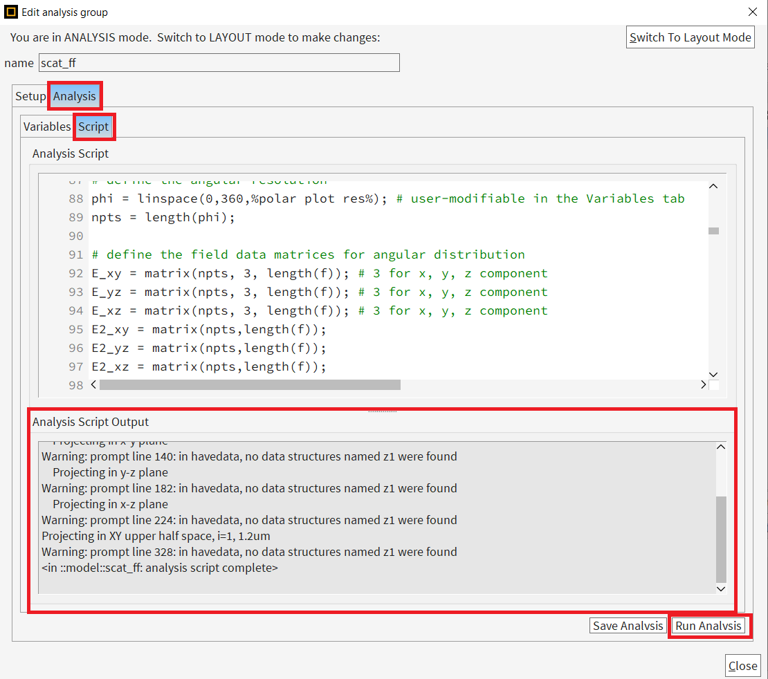
You are welcome! Would you be able to share a screenshot of the error? If you edit the Analysis Group, then click check the code at the two places (Setup-->Script) and (Analysis-->script), you will see an option called "Run Analysis". After finishing the simulation, if you click on that it will give you output messages as well as error messages. 

I would be interested to look at the screenshots of the error messages. Thank you!

Regards,
Amrita

[pnair]

Please find the attached screenshot of the error here.

[Amrita Pati]

Thanks for sharing the screenshot, Prabha!

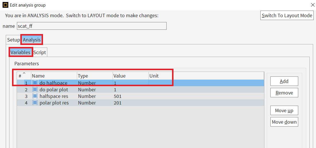
Is the following variable (do halfspace) set to 1 in your Analysis Group?

Regards,
Amrita

[pnair]

Please find the attached screenshot of the analysis group here.

 

[Amrita Pati]

[Amrita Pati]

To perform the XY halfspace projection, set the first variable: do halfspace to 1. It is currently set to 0, so the analysis group is not performing the calculation.

Regards,
Amrita

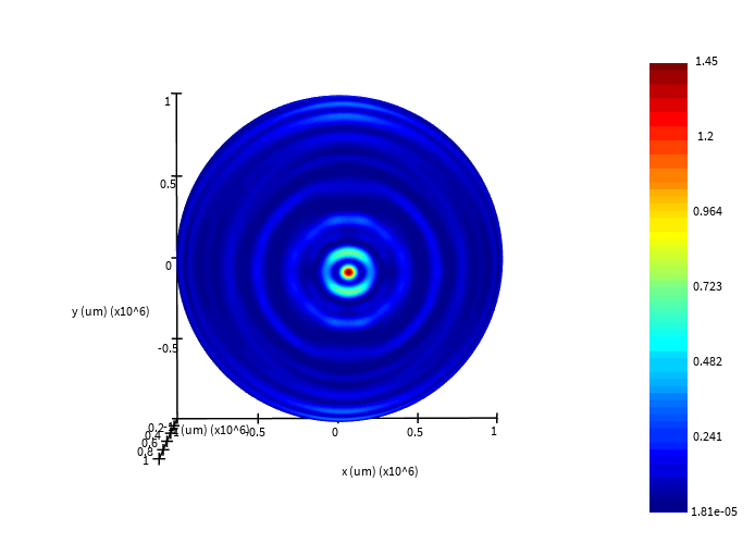
[pnair]

Thank you Amrita for the corrections made to the script. I run the simulations using this corrected script. This is what i have generated using the script for box of 5 monitors

And, This is the plot that i have generated using one large z-normal monitor.

How can I make the first plot more better? Is there any way, may be changing the resolution of the simulation to get more clearer plot?

[Amrita Pati]

It's good to see that the results are very similar! That is true, the default resolution is low and the graph looks pixelated. If you look at the last screenshot I shared, there is a variable (third in the list) called "halfspace res". You can increase this to improve the farfield resolution. I had my set as 501, which might not be necessary and will probably take a minute or so. You can start at a lower value like 201 and see what the plot looks like.

Regards,
Amrita

[pnair]

Hello Amrita,

I have already changed the resolution of the halfspace and polarplot as shown below, based on your previous discussion:

I have got this plot and this seems to be better than the first one.

[Amrita Pati]

That's great to hear! It does look better. Please feel free to let me know if there are any further questions.

Regards,
Amrita

[pnair]

I have a question related to changing/increasing the value of resoulutions:

1) half space res- 31 to 201

2) Polar plot res - 21 to 201

What does it exactly doing and how the polar plot in the visualize is changing or become more clearer? Is it similar to changing the resolution in farfield settings window?

 

[pnair]

And 201 is enough to get a clearer plot or do i need to increase to more higher values?

[Amrita Pati]

When you plot the the farfield on a plane, the resolution tells us how many points in the plane the fields are calculated at. The more the resolution, the more is the number of points in the farfield plane. For example, my resolution was 501, so my grid in the farfield is 501x501.

Is it similar to changing the resolution in farfield settings window?

That is correct! It is the same thing.

And 201 is enough to get a clearer plot or do i need to increase to more higher values?

I think it's upto you. If you don't see significant changes in the plot after a certain resolution (and you see the expected result), then there is no need to increase the resolution further as it is just going to increase the calculation time.

Regards,
Amrita

[pnair]

 

Thank you for the reply.

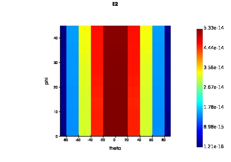
I have a question related to the data generated from XY_half space. Is it possible to use a script to generate a data in the from grid of theta and phi angles using the following script so that I can plot the data in a more better form. And what should I give for the monitor name here as we have box of 5 monitors in this case?

 

m="Monitor1";  # Monitor name
res = 201;    # projection resolution
E2 = farfield3d(m,1,res,res);
ux = farfieldux(m,1,res,res);
uy = farfielduy(m,1,res,res);
theta = linspace(-90,90,100); 
phi = 0;
plot(theta, farfieldspherical(E2,ux,uy,theta,phi) ,"theta", "E^2", "E^2 at phi=0");

 

Interpolate field data to a grid of theta and phi angles.

 

theta = linspace(-90,90,10);
phi = linspace(0,45,11);
Theta = meshgridx(theta,phi);
Phi = meshgridy(theta,phi);
E2_angle = farfieldspherical(E2,ux,uy,Theta,Phi);

[pnair]

Hello Amrita,

I have a question related to the data generated from XY_half space. Is it possible to use a script to generate a data in the from grid of theta and phi angles using the following script so that I can plot the data in a more better form. And what should I give for the monitor name here as we have box of 5 monitors in this case?

[Amrita Pati]

Hi Prabha,

We can collect the fields from the analysis group rather than from the monitor. I would try something like this:

theta = linspace(-90,90,100); 
phi = 0;
Theta = meshgridx(theta,phi);
Phi = meshgridy(theta,phi);

XY_halfspace = getresult("scat_ff","XY_halfspace"); #getting the result from the analysis group combining farfield from 5 monitors
ux = XY_halfspace.ux;
uy = XY_halfspace.uy;
E2_upper = XY_halfspace.E2_upper; #E2 is intensity
plot(theta, farfieldspherical(E2_upper,ux,uy,theta,phi) ,"theta", "E^2", "E^2 at phi=0");

I just modified the code you shared here. So, I haven't actually tested it. Please feel free to let me know if you see any issues. Thank you!

Regards,
Amrita

[pnair]

Hello,

I tried to run this code. But, I can't generate a grid of data. This is the grid of theta and phi angles generated by the code for one monitor as following:

m="Monitor1";  # Monitor name
res = 201;    # projection resolution
E2 = farfield3d(m,1,res,res);
ux = farfieldux(m,1,res,res);
uy = farfielduy(m,1,res,res);
theta = linspace(-90,90,100); 
phi = 0;
plot(theta, farfieldspherical(E2,ux,uy,theta,phi) ,"theta", "E^2", "E^2 at phi=0");

 

Interpolate field data to a grid of theta and phi angles.

 

theta = linspace(-90,90,10);
phi = linspace(0,45,11);
Theta = meshgridx(theta,phi);
Phi = meshgridy(theta,phi);
E2_angle = farfieldspherical(E2,ux,uy,Theta,Phi)

But, with the above-mentioned code for XY-half space, i can only generate the following plot

But, i need to generate a grid of theta and phi as mentioned in the 1st plot. So, is there any way to generate a grid plot from the above mentioned script for xy_half space?

 

[Amrita Pati]

I shared the code for the phi = 0 plane (the first code snippet you had shared), therefore, you can modify to include the entire theta-phi plane:

theta = linspace(-90,90,201);#Choose the range of theta interested in 
phi = linspace(0,45,201);#Choose the range of phi interested in
Theta = meshgridx(theta,phi);
Phi = meshgridy(theta,phi);

XY_halfspace = getresult("scat_ff","XY_halfspace"); #getting the result from the analysis group combining farfield from 5 monitors
ux = XY_halfspace.ux;
uy = XY_halfspace.uy;
E2_upper = XY_halfspace.E2_upper; #E2 is intensity
E2_angle = farfieldspherical(E2_upper,ux,uy,Theta,Phi)

image(theta, phi, E2_angle);

Edit: Changed E2 to E2_upper in the highlighted text.

Regards,
Amrita

 

[pnair]

Thank you for the code. I run the simulation and generated polar plots. I have a question related to the position of the monitor. As I am using box of monitors, all the monitors are on the thin film which I am simulating. 

Here, Z1 monitor, which is the top monitor is on the film. But, as I was going through this article "https://optics.ansys.com/hc/en-us/articles/360034395194-Changing-the-far-field-refractive-index-analysis-object". As my monitors are on the film, is this farfield analysis group is considering the refractive index of the vaccum or is it extending the substrate to the infinity? So, how can validate my results?

 

[pnair]

Hello Amrita,

Thank you for the code. I run the simulation and generated polar plots. I have a question related to the position of the monitor. As I am using box of monitors, all the monitors are on the thin film which I am simulating. 

Here, Z2 monitor, which is the top monitor is on the thin film. But, as I was going through this article "https://optics.ansys.com/hc/en-us/articles/360034395194-Changing-the-far-field-refractive-index-analysis-object". As my monitors are on the film, is this farfield analysis group is considering the refractive index of the vaccum or is it extending the substrate to the infinity? So, how can validate my results to see if this method is correct?