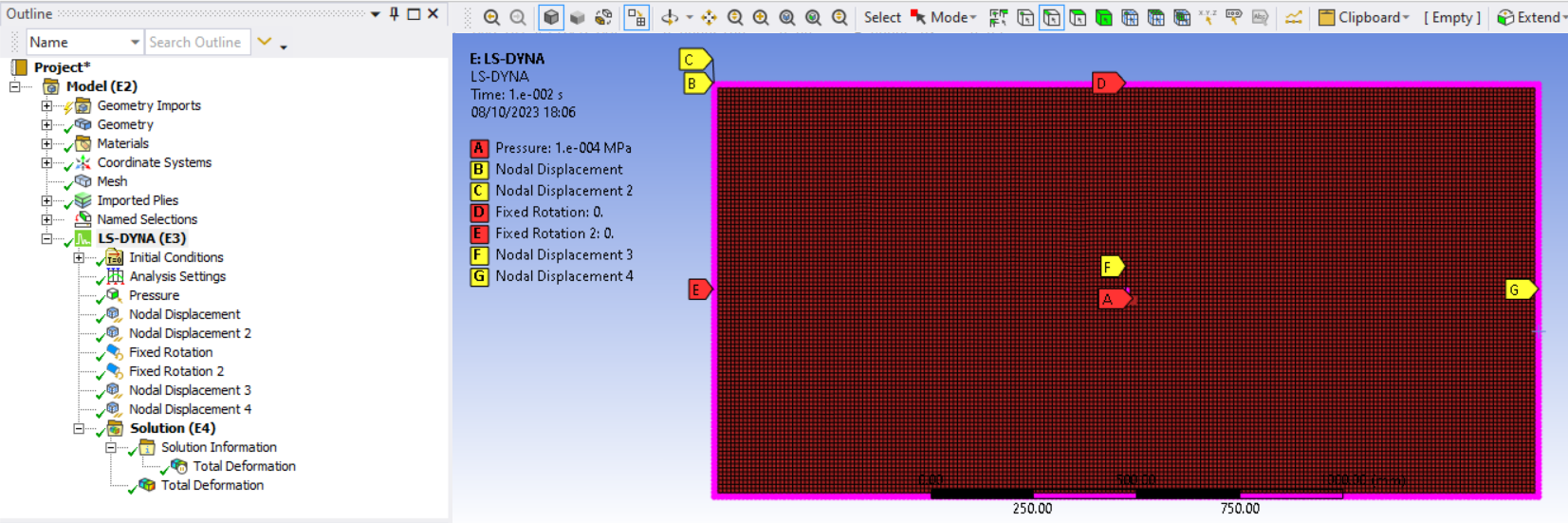
-
-
October 8, 2023 at 3:14 pm
AhmetKaya
SubscriberGreetings,ÂI'm working on a project focused on analyzing the quasi-static compression behavior of Miura-ori structures made from paperboard. Initially, I planned to use LS-DYNA for this research. However, before diving into that, I decided to compare different solvers—static, explicit dynamic, and LS-DYNA—on a simple composite plate.ÂI followed a YouTube tutorial (&t=458s) and found that when I used the static structural solver, my results matched the video perfectly. However, when I tried the same with LS-DYNA and the explicit solver, my results and deformation behavior didn't align with the video. (The only difference in the models are in static structural there is nodal ratation boundary condition, whereas, since there is not such BC, I defined my rotation constraint as fixed rotation in explicit dynamics and LS-Dyna analysis)ÂI'm currently investigating the cause of this discrepancy. Could it be that the ACP module isn't transferring data correctly to the explicit dynamic and LS-DYNA solvers? Here's a quick summary of my modeling process and results:ÂÂAny insights would be greatly appreciated.ÂWarm regards,Ahmet K.
Â
-
October 10, 2023 at 10:27 pm
Reno Genest
Ansys EmployeeHello Ahmet,
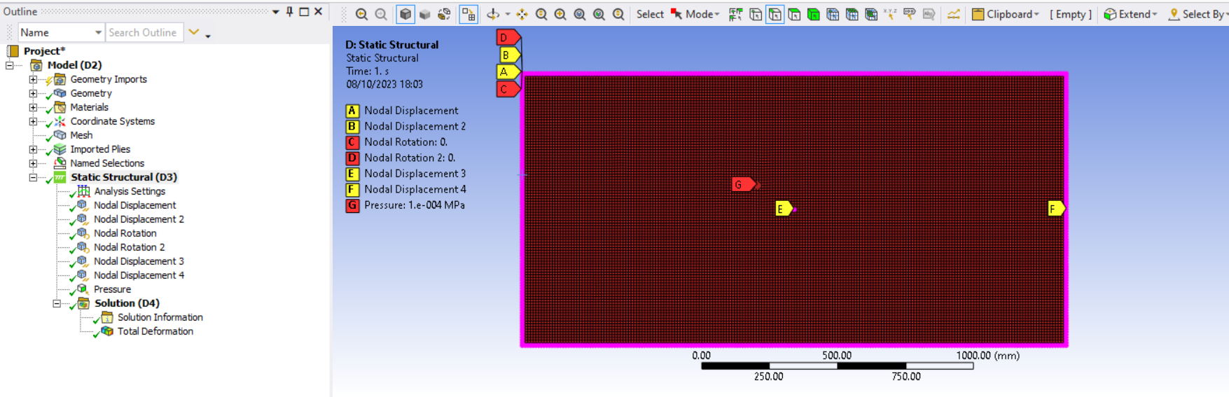
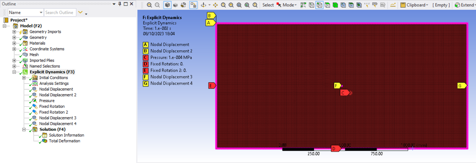
If the boundary conditions are not the same, you will get different results. Have you tried to fix the rotations in Static Structural as well? What result do you get?
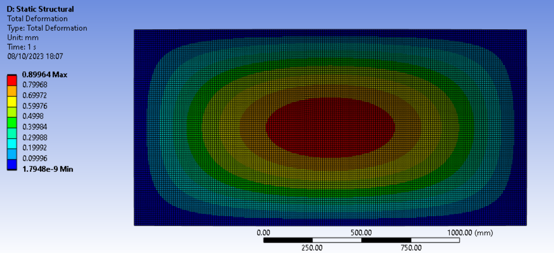
Also, implicit and explicit are different simulations and results are often different. In implicit, you calculate the static equilibrium position and do not consider the inertial effects (F=ma). In implicit, the time at the end of the simulation is not important (the default is 1 second, but you could use 100s and get the same result).Â
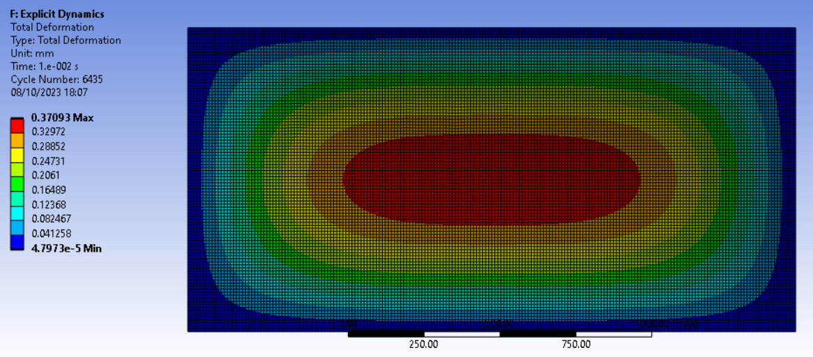
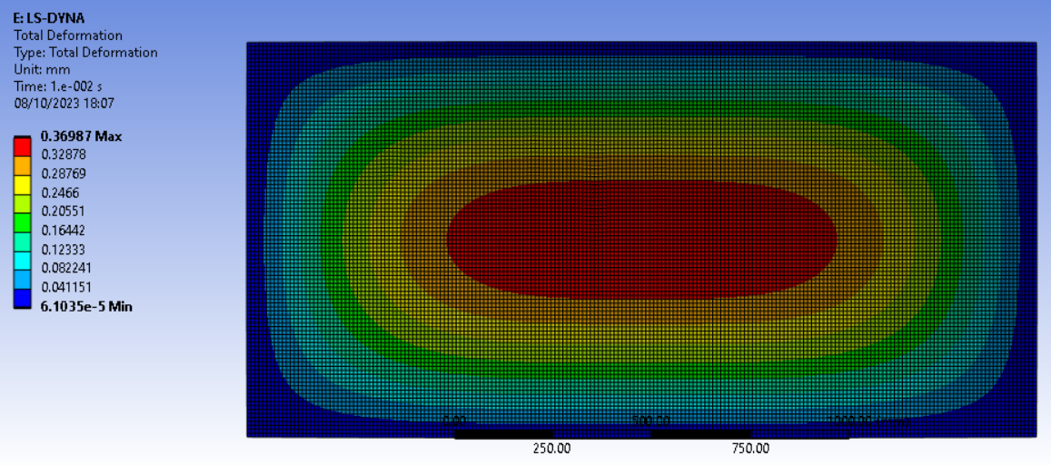
In explicit, the inertial effects (F=ma) are taken into account and time matters. If you apply the load at different speeds you will get different results. Also, if the part is fully constrained and there is no rigid body motion, then the deformation solution will vibrate around the equilibrium position in time. If you have damping, the solution should eventually settle a the equilibrium position.Â
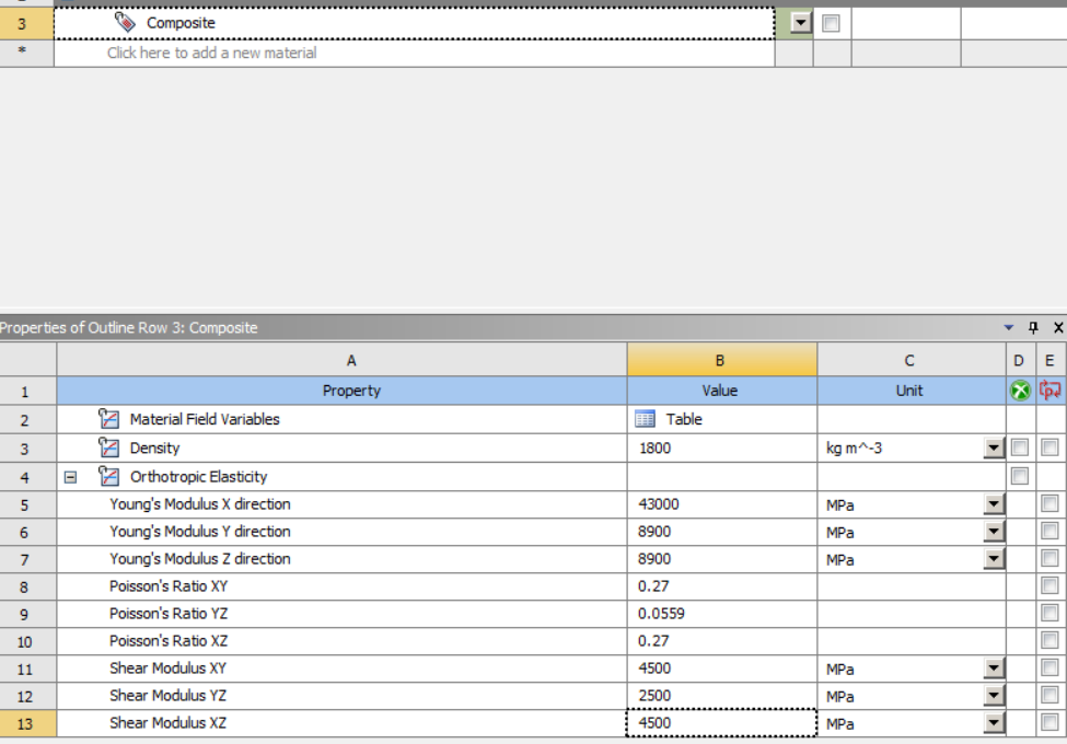
If you wonder if the composite information is transferred properly in explicit, please try to run the same model with the default "Structural Steel" material in Workbench. Remove the composite layup and compare the results. I bet the results will still be different in implicit vs explicit because the boundary conditions are not the same.
You will find more information about implicit vs explicit here:
/courses/index.php/courses/time_integration/
Let me know how it goes.
Â
Reno.
Â
Â
-
October 11, 2023 at 6:53 am
AhmetKaya
SubscriberHi Reno Genest,
Thanks a lot for your detail explanation. I will go through your suggestions, and hopefully find something useful. As far as I understand from your explanation eventhough BCs seems to be same, the inertial effect consideration affects the solution. In order to find similar results, I must add damping and increase the solution time so that applied load speed will be small enough so inertial effects will be minimized. Yet, this will increase the solution time.Â
Thanks a lot again,Â
BR,Â
AhmetK.
-
- The topic ‘Modeling composite in ACP using solvers STATIC vs Explicit Dynamic vs LS-DYNA’ is closed to new replies.
-
3977
-
1461
-
1272
-
1124
-
1021
© 2025 Copyright ANSYS, Inc. All rights reserved.