Learning Forum

[evanmehedihasan]

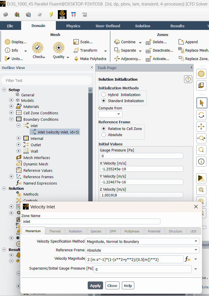
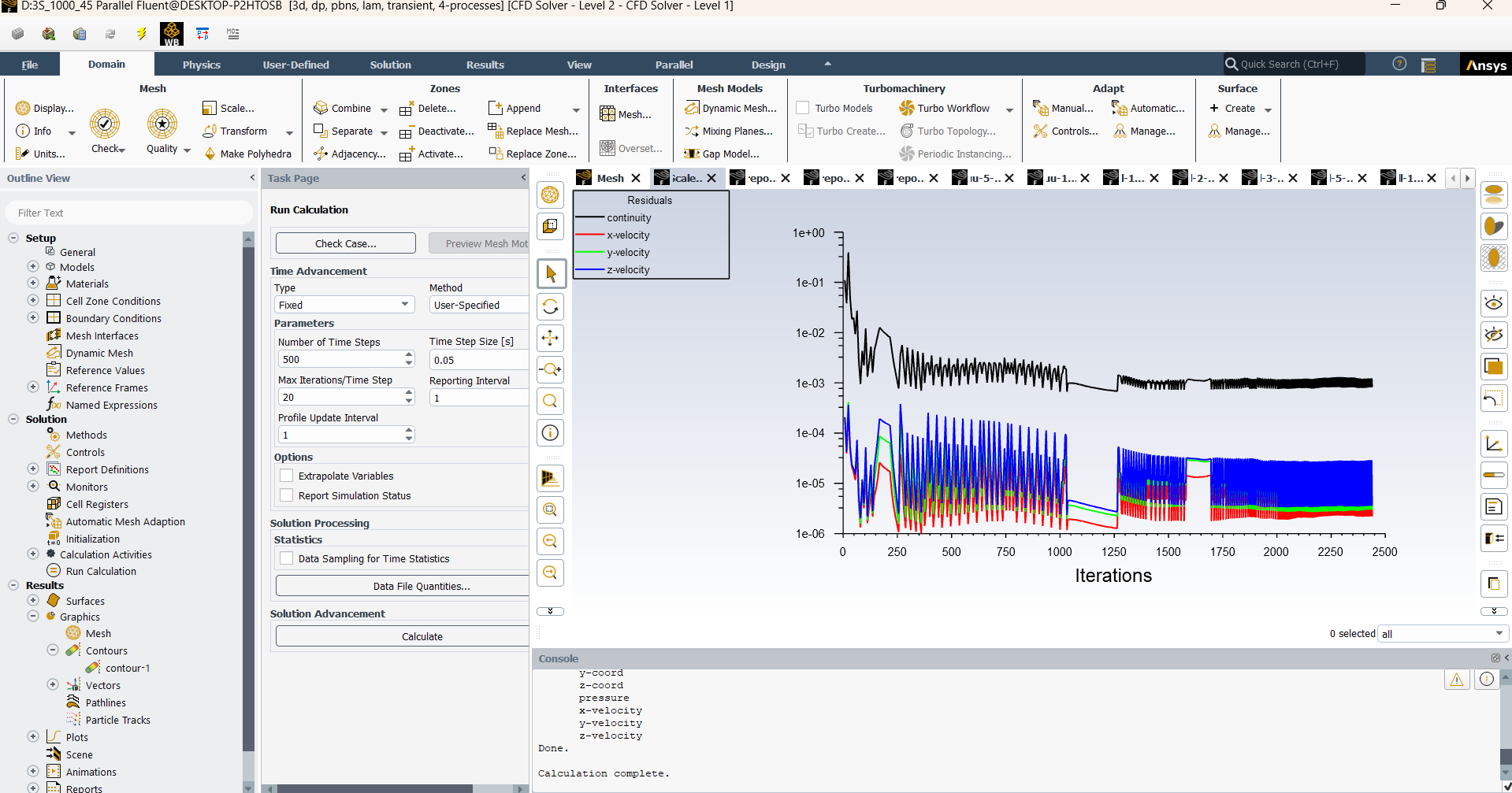
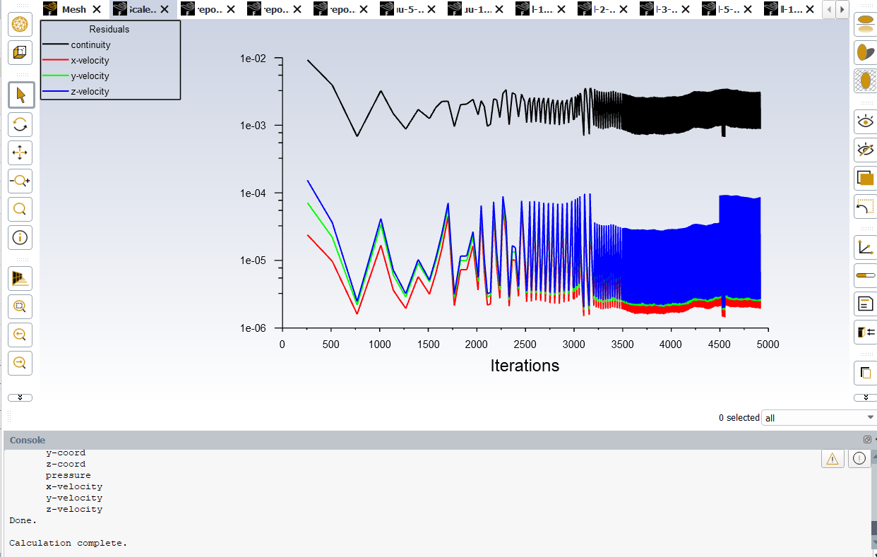
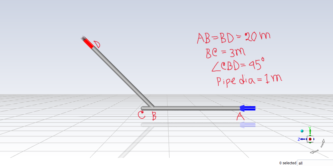
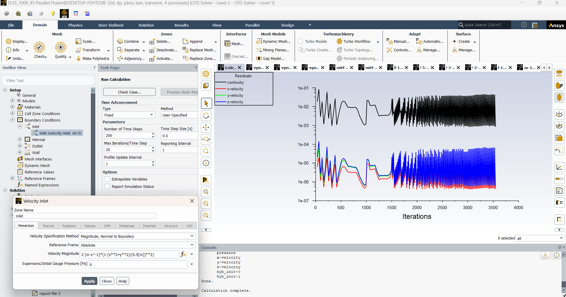
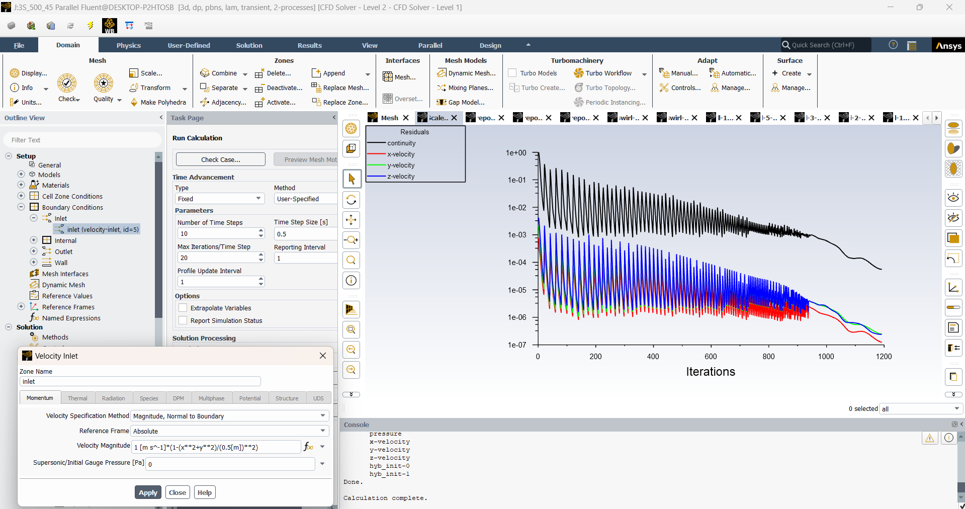
Greetings everyone. I am a new user of Ansys and I have very little knowledge about that software. Currently, I am trying to perform a simulation of laminar flow through a blind wye pipe as you can see in image 1. The diameter of the pipe is 1 meter and I have set the kinematic viscosity as .001 m/s. In the inlet, I have inserted a parabolic velocity profile. The outlet boundary condition is set to outflow. I have used transient laminar model for solution. Now the issue is, when, my average velocity is 0.5 m/s (Max velocity- 1m/s), the Reynolds number is 500 and the solution converges like image 3. But when the average velocity is 1 m/s (max velocity- 2 m/s), the Reynolds number is supposed to be 1000 and this time the solution doesn't converge (image 2) if I use the laminar model. Why does that happen? Is is cause the recirculation of fluid in blind part causes the flow to go turbulent? And even if it does, how can I know upto which inlet velocity, the flow remains laminar? And also how can I determine the Reynolds number where the flow suddenly become turbulent although it started off as laminar?

[NickFL]

Why are you running the simulations in transient? What did you use as an initial condition? It is always good practice to start from a converged steady-state solution to "help" the solver find the correct solution.

My first guess is that the 0.5 [s] is too large a time step to capture any unsteadiness in the higher velocity case.  Compare the velocity profiles from two different times. Where are the areas where there are significant differences? If you were to decrease the time step size, you may be able to better capture the unsteadiness. Yes laminar flows can be unsteady.

Think back to y = sin(x) . If you have too big a step in x then you won't recoginze the curve that appears. A similar thing happens when solving an unsteady problem. We and the solver need to be able to resolve the unsteadiness by decreasing Dt. 

[evanmehedihasan]

Hello NickFL, I initialized the flow from the inlet (Vx=Vy=0 ms, Vz=1 m/s) as you can see in image 1. I also reduced the step size to 0.05 (in the case of Re=1000) as you suggested which brought me a more stable result compared to before (Image 2). But the oscillation is again more prevalent where the Reynolds number is 1500 (Image 3). The residual of continuity equation doesn’t fall below the 10^-3 and the curve remains flattened out. Would you say this solution where the residual curve behave like that is acceptable? Or it not, what would you further suggest me to do?

     

 

        

[NickFL]

Let us go back to my first reply. Is there a reason why you are running this in transient? Second your initial condition is not great, that is why the first timesteps are not converged. You should definately not consider these in your final analysis. One thing to do would be to increase the maximum number of iterations per timestep. But a better approach would be to use a steady-state solution as the initial condition.

On your question whether the residual curve is acceptable, that is just one data point to determine convergence. Simply looking at the residuals is not enough to determine if the solution is good enough. You should have other monitors that will help you determine if the solution is "good enough". Without knowing your problem it is difficult for any of us to recommend what monitor points you should include. That is why I asked above why are you running it as a transient solution. Usually the first step is to solve the steady solution.

[evanmehedihasan]

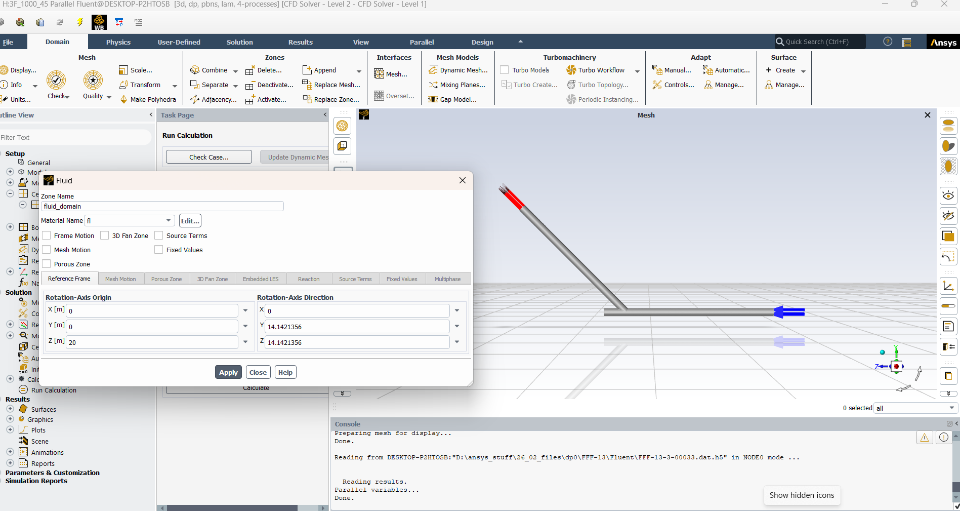
Hello, I ran the simulation again in steady state with a better mesh quality and it converged. Turns out, my mesh quality was too poor to reach convergence. Now I have two more questions. Those are  to check whether I am wrong or not. The fluid enters as irotaional flow in the inlet. But after the flow is hindered by the blind part of the pipe, small vortices are created in the inclined part (CD) (image 1). I wanted to measure that by using swirl number.

1. So if I am to calculate swirl nummber in the CD part (20 meters) of ther pipe, please comfirm me if I have defined the rotaional axis properly (Image 2) ? I have defined my rotaional axis as the axis of the CD part of the pipe. Where the coordinate of C is (0,0,20) and of D is (0, 20*sin45, 20+20*cos45) or (0,14.142, 34.142).
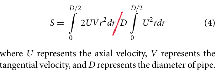
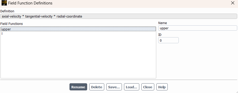
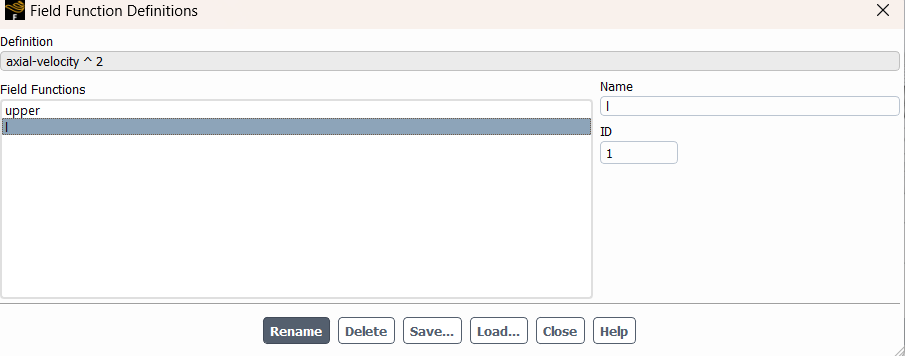
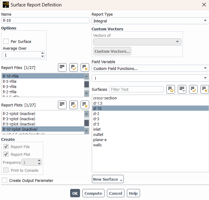
2. The definition of swirl number says it's the ratio of axial flux of the angular momentum to the axial momentum (Image 3). Now, to measure the number, I have used the custom field function to define the intrgrand of the numerator and denominator (image 4,5). Then I integrated them in surface field report (Image 6,7). and finally determined the swirl number in (image 8). So, I was wondering if my process is right or not.

 

[evanmehedihasan]

.