Reply To: Calculate EQE in CHARGE

[handon]

Hello, khashayar. It's been a long time. 

Your replies were helpful for me and I have tested a lot of simulations.
Here's a new question with my latest progress.

---------------------------------------------------------------------------------------------------------

I have a question about running CHARGE simulation with scripts.

 

My final goal in this simulation is plotting spectral EQE at 300~1100 nm wavelength range.

I’m now testing my simulation including script file at 300 ~ 305 nm.

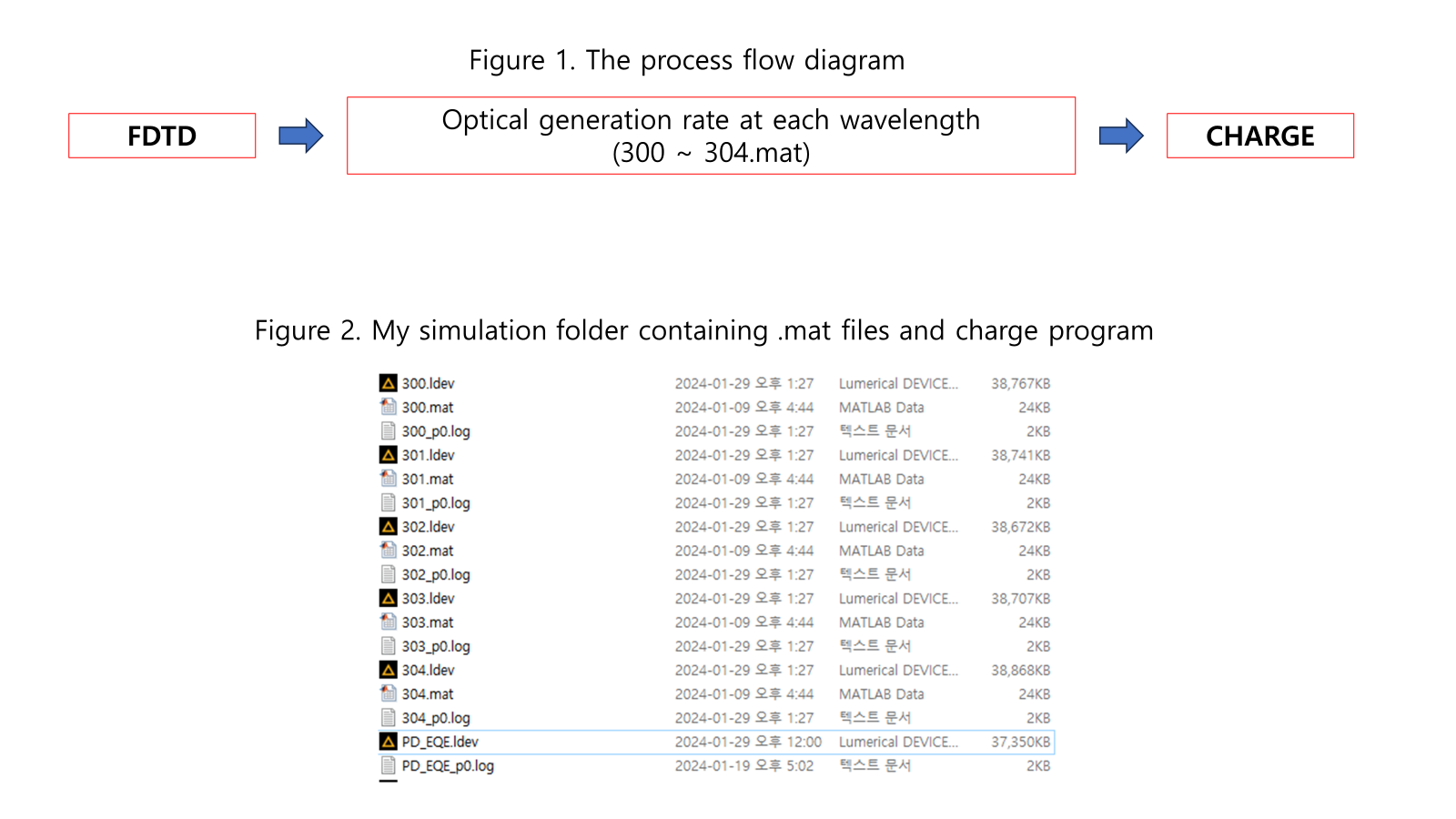
The process to plot spectral EQE is as follows (Figure 1):

 

At first, I run the FDTD and generate .mat files that contain optical generation rate (G vs. x, y, z) at each single wavelength.  (It was conducted by the script of analysis group in FDTD.)

Now, these .mat files (300 ~ 304.mat) are ready to import from script in CHARGE. (Figure 2)

 

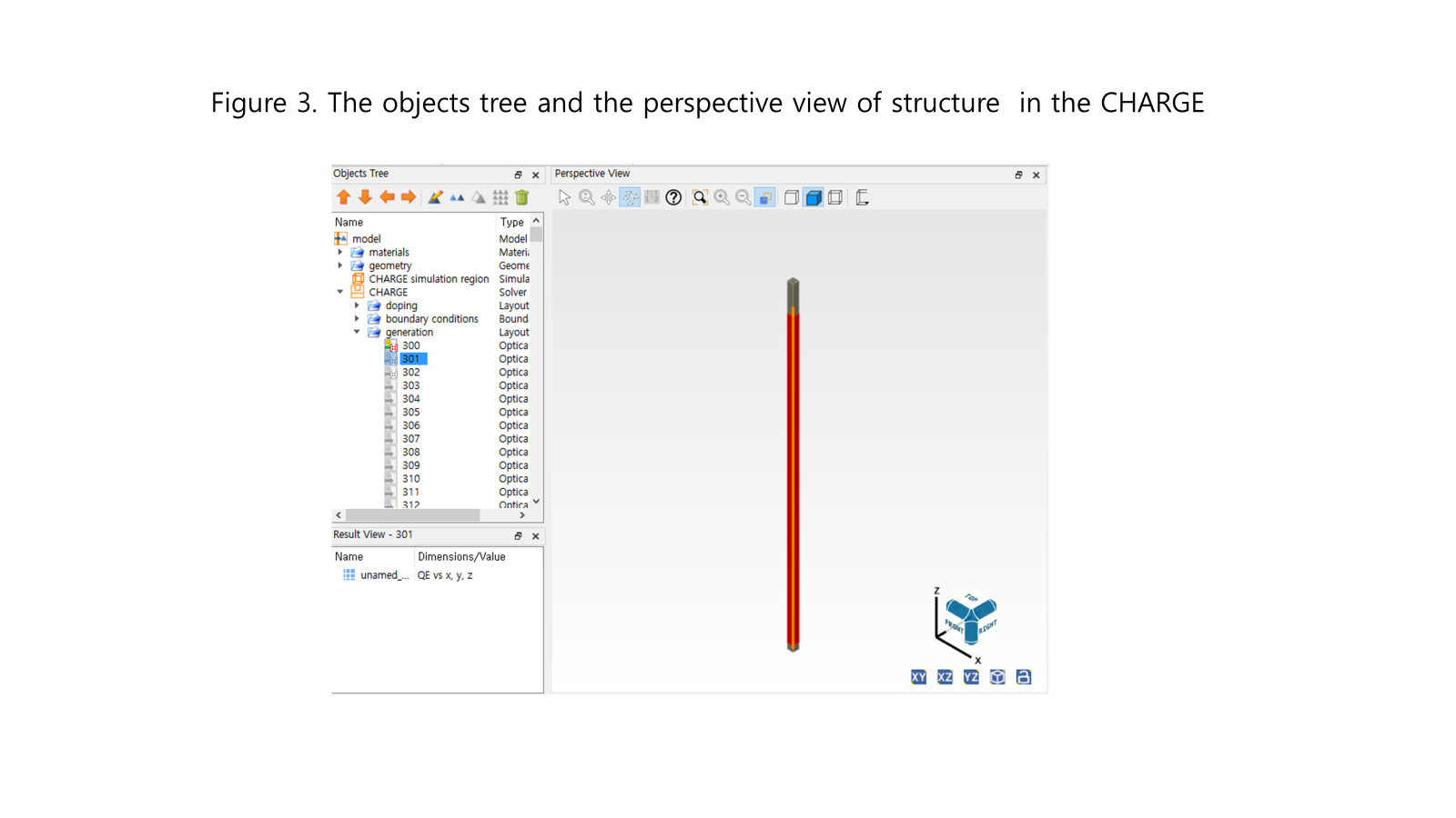
In CHARGE, there is a generation folder that has optical generation imports named with 300 ~ 1100. (Figure 3)

Run the script and get result.

The script file is modified from cis_QE.lsf in the below example:

CMOS - Cross talk and QE extraction – Ansys Optics

 

However, there are some problems in the CHARGE step of process.

.mat files could not be imported by script. In the script, .mat files are imported by ‘importdataset’ command. But, the script result shows that very low Jsc, and it would might be dark current. It means optical generation rates are not successfully imported.

 

I’m not sure that my script is optimized.

I put a lot of effort into calculating spectral EQE, but it still hard work for me.

If you have any idea on the script or script codes for calculating EQE, please give me some advice.

 

The whole codes in this script are shared below:

 

##########################################################################

# Scriptfile: cis_QE.lsf

#

# Description:

# This file runs a sweep over all generation objects for each angle

# and calculates efficiency and cross talk

#

# Copyright 2012, Lumerical Solutions, Inc.

###########################################################################

 

start_wl = 300;

end_wl = 304;

npts = end_wl - start_wl + 1;

surface_area = getnamed("CHARGE simulation region","x span")*(getnamed("CHARGE simulation region","y span"));

Jsc = linspace(0,0,npts);

 

clearjobs;

original_filename = currentfilename;

for (i = start_wl:end_wl) {

select("CHARGE::generation::"+num2str(i));

importdataset(num2str(i)+".mat");

groupscope("::model");

generation_object_name = num2str(i);

groupscope("CHARGE::generation");

selectall;

set("x",0);

set("y",0);

set("z",0);

set("enabled",0);

setnamed(generation_object_name,"enabled",1);

filename = num2str(i);

save(filename);

addjob(currentfilename);

 

?"Added " + currentfilename;

groupscope("::model");

}

load(original_filename);

 

?"Running sweep...";

 

 

runjobs;

 

##########################################################################

?"Processing results...";

 

for (i = 1:npts) {

load(num2str(299+i));

filetag = "wavelength" + num2str(299+i) + "nm";

Jsc(i) = pinch(getdata("CHARGE","emitter.I")/surface_area*0.1);

}

 

load(original_filename);

 

print(Jsc);

wl = linspace(start_wl,end_wl,npts);

EQE = (-Jsc*1239.8)/(100*wl);

 

plot(wl,EQE,"wavelength", "EQE %");

setplot("y min",0);

setplot("y max",1);

legend("");