Reply To: Adjoint Method for Optimising Diodicity of Tesla Valve

[Akram Radwan]

Hello Jason,

Let me try to reconstruct what was lost because of the database corruption. This time I have a local backup.

 

General recommendations

Do not use Ansys Workbench for shape optimization. You can prepare your calculations there. But the automation of WB can conflict with the various files the optimizer creates. I strongly recommend using the standalone version of Fluent for the optimization.

Do a sensitivity study before running the optimization. Note that Fluent can only post-process the sensitivity fields of the current calculation. To compare them, you need either separate sessions or export the results to EnSight to have both loaded at the same time. This analysis has multiple goals:

• Understand which regions of which operating condition are sensitive.
• Understand how different observable definitions might influence the result.
• Understand if or where observables support each other or are conflicting.

You can explore different optimization strategies:

• Explore different observables. Some might work better than others. For example, the velocity magnitude does not have a sign and can be maximized or minimized for the two directions. The mass flux has a sign and must be treated differently. For other boundary conditions you might need the pressure drop but measuring the total pressure drop between inlet and outlet or the pressure drop in one of the channels can lead to different results.
• You can apply a split optimization strategy. First, optimize the forward path on its own. Then optimize the reverse direction on its own. This simplifies the optimization process. Depending on the sensitivity distribution, you might want to restrict the deformability of certain regions.
• With the upcoming 2025 R1 (available in January), you can test if the optimizer can keep the mass flow rate in the forward direction above a user-defined minimum and minimize it in the other direction.

Also keep in mind that you have sharp corners in your geometry. The separation at these corners is often transient in nature, which influences the stability of the adjoint calculation more than it influences the stability of the flow calculation. The residual minimization scheme can often bring the adjoint residuals down. But you should be sure that the flow calculation is stable, i.e., stopping the flow calculation at different iterations does not show a different flow field. There are averaging methods available if this cannot be achieved but I do not recommend them before you have more experience with more stable flow calculations.

 

Boundary conditions

You have two possibilities for your BC types. You can use two pressure inlet BCs or a combination of mass flow/velocity and pressure outlet BCs.

The advantage of the pressure inlet BCs is the easy way to parameterize them. Don’t get confused by the name, when the flow goes out of the pressure inlet it behaves just like the pressure outlet BC type. You might need to initialize the flow calculation between the optimization steps, though. And two pressure BCs are not the most stable setup to begin with.

The advantage of mass flow inlet or velocity inlet and pressure outlet BCs is their stability. However, changing the BCs in an automated process is not available as a built-in method in Fluent. You need a few lines of script to do this.

But the choice of BC should be driven by what you want to model. The Tesla valve should choke the flow for the reverse direction. While it is doing this regardless of the boundary conditions, the outcome for the optimization can be very different. For pressure BCs the mass flow rate reduces, which can change the flow behavior (e.g., the existence or strength of recirculation and separation). For mass flow/velocity + pressure BCs the pressure drop changes but the general flow behavior is unlikely to change.
Consider the true operating conditions that apply to operating the device. There might be more than just the two general flow directions.

I outlined the script to change the BC-type in the other thread if you need that. Because of the limitations of scripting support especially for Scheme, I cannot provide more details. When you have difficulties, test the script line by line before using it within the optimization loop.

To initialize the flow and/or adjoint solution, search the documentation for “;@”. You can find it in the Fluent 2024 R2 User’s Guide, III. Solution mode, chapter 48.2.6. Using the Gradient-Based Optimizer, step 10: https://ansyshelp.ansys.com/public/account/secured?returnurl=/Views/Secured/corp/v242/en/flu_ug/flu_adj_usage.html%23flu_adj_sec_adjoint_grad_opt
Add a new execute command using “Execute Repeatedly every 1 Design Iteration” with the following three lines:

/solve/initialize/hyb-initialization yes
/adjoint/run/initialize
;@before-flow

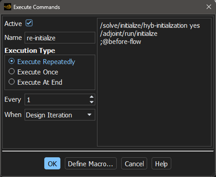
Depending on your strategy and operating conditions you might want to split this into two commands to initialize flow and adjoint separately at different steps of the optimization process.

Note: 2025 R1 will initialize automatically when you have more than one objective.

 

Adjoint convergence

From what you have shown, I’m not concerned about the adjoint convergence. The residual minimization scheme can reduce the adjoint residuals quite reliably. If it struggles, you can increase the number of modes.
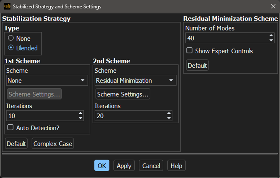
Important: Never show the expert controls of the residual minimization stabilization scheme! Just having this box checked can change the behavior of the stabilization! Only use it when you know how it influences the calculation.

Typically, I use Solution-Based Controls Initialization to reset the solver controls on initialization, 10 iterations for the first scheme without auto detection, and 20 on the second. That should be enough to converge the adjoint. If it’s not, increase the number of modes slowly. If you ever need values above 140 it’s time to think about alternative strategies and closer examination of the flow and adjoint solutions. For a better understanding, I recommend the training material for the gradient-based optimization that is available on the Ansys Learning Hub.

I also recommend taking a closer look at the flow behavior when you have convergence difficulties with adjoint. Do you have separation or recirculating flow somewhere? If yes, is this stable when you stop the calculation at different iterations or does it change slightly?
There are advanced diagnosis tools available in the text interface by keeping the cell residuals for the flow and the adjoint calculation, if you really want to dive deeper into understanding what is happening. I do not recommend this step. It requires a lot of experience to make sense out of the values that you see there. But it does exist if you want to analyze the stability on a cell level. Search the User’s Guide for “cell residuals” for the flow solver and check chapter 48.2.3.4. Printing and Postprocessing the Adjoint Equation Residuals for the adjoint solver. Again: I do not recommend this unless you have a lot of time to gain understanding of how to interpret the results with many different cases.

 

Sensitivity analysis

Taking a closer look at the shape sensitivity is often ignored but it can give you valuable insights. The quantities you want to look at are the log10 shape sensitivity or the surface shape sensitivity. The first one is a logarithmic scale of the shape sensitivity, which makes it easier to see the distribution because it has a very large range. The second one is a smoothed version of the shape sensitivity.

I recommend to start with the surface shape sensitivity but before you do, change the postprocess options that you can access from the Design ribbon. Make sure the surface shape sensitivity is set to spring. The default radial basis function approach can be computationally expensive. Whichever method you use, this is just to get an impression of the sensitivity distribution, it is not used for anything by the mesh morphing. The Design Tool uses the raw shape sensitivity and applies the smoothing during the morphing process, which depends on the selected morphing method.
Unfortunately, it is not possible to export the surface shape sensitivity vector components to EnSight. If you want to use EnSight for a direct comparison, use the unsmoothed shape sensitivity components instead.

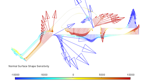
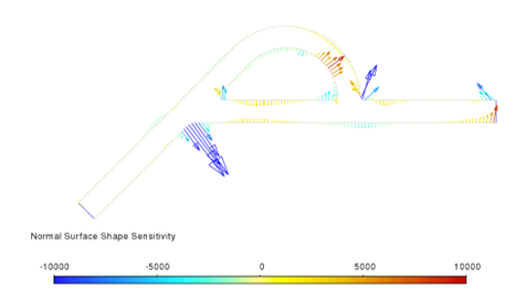
Use vector plots for 2D cases. For 3D cases it is often more convenient to start with contour plots of the normal surface shape sensitivity. Check the regions of high absolute values for both flow directions.

• Are the regions similar?
  • If yes, is the sign identical (general direction of the vector)?
    • If yes, both observables support each other, it’s just a question of scaling them appropriately.
    • If no, either the observables are in conflict with each other. Optimization without defining trade-offs is either very challenging or even impossible.
  • If no, how different are they? Would it be possible to concentrate the shape change of one flow direction to certain regions and the reversed direction to different ones?
• How different are the absolute values of the shape sensitivities?
  • Remember that the shape sensitivity has a unit that depends on the selected observable. If the observables are comparable (e.g., both use the average velocity magnitude at one boundary), differences indicate how to scale the objectives.

Based in the outcome of looking at the shape sensitivities you can derive an optimization strategy.

Remember: depending on maximizing or minimizing the observable, you might need to reverse the direction of the sensitivity vectors!

 

Optimization strategy

As indicated initially, there are different strategies possible. The flexibility of the optimizer is limited in favor of a fully automated workflow. Depending on the strategy that you want to use, you might need to do this manually.

Standard approach
Based on the sensitivity analysis, you can set you objectives and hope for the best. While this works well for a single objective, it rarely works for multiple objectives or conditions.

Consecutive optimizations
This approach works best when the sensitivities have their extreme values in different regions of the domain. It is mostly useless when they are in conflict everywhere. Just run the optimizations with a single objective/condition. Once this cannot be continued, change the flow direction and run a new optimization.
You can also change the region easily with this approach, for example, to optimize the straight part of the pipe for the forward calculation and the bended part for the reversed direction.

Customized approaches
Obviously, there are more approaches.

Similar to the consecutive approach from above, you could do this in one step. There is no tool in Fluent to automate this apart from writing your own full optimization script. The idea is to set the first condition, calculate flow and adjoint, set the region and design conditions as needed, and morph the mesh. Then switch to the second condition and repeat. With this alternating approach you can run a combined optimization but with different settings for the mesh morphing.

You can also use different observables for the directions. I didn’t test this. But you could come up with an idea to maximize the flow rate through different parts of the domain, e.g., for the reverse direction maximize the flow rate through the bend, for the forward direction maximize the flow rate through the outlet. You can implement this in the optimizer by setting an objective to ‘none’ for the condition where it is not relevant. This will still calculate the adjoint for it, but it is not considered during mesh morphing.

As indicated above, 2025 R1 offers new methods for the optimization that can be useful for a case like this. You can implement a similar procedure yourself. Just run a single-objective optimization but stop it when the observable for the other operating condition is outside the bounds (e.g., the mass flow rate for the primary flow direction drops below a user-defined minimum). Only if this is the case, optimize for the other direction until it is well above the threshold. Then continue with the first set of settings.

There are more. I hope you get the idea that there is not just the workflow that is implemented in the gradient-based optimizer. That is the most common one, but not the only one. Understand the sensitivities. Then derive a workflow to change the shape in a promising way.

 

Conclusions

Optimizing a Tesla valve design is not the most trivial task.

1. Start with the boundary conditions. Which ones are reasonable to describe the physics of the problem?
2. Shed a thought or two about local stability of the flow calculation.
3. Think of possible observables. There are often more than one possible objective functions and because of the nature of the adjoint method the resulting shape can be quite different.
4. Analyze the sensitivities for the different operating conditions and observables. Understand where they support each other and where they are in conflict.
5. Derive possible optimization strategies. Not all of them are available as built-in capabilities. Be creative, then simplify.
6. Run the optimization. Analyze how it performs. Fine-tune the approach or use one of the other strategies.

I hope I didn’t miss a question and that I covered all of the lost information.