Learning Forum

[José Mantovani]

Hello everyone. Well, the publication aims to resolve doubts about the results obtained by FLUENT when compared to experimental results, I share with everyone for general understanding.

The flow in question is the flow through the divergent channel, backward facing step geometry. The simulation is based on the experimental study of Jovic and Driver (1994), an experimental study carried out to serve as a basis for numerical analysis. From this, we have the computational domain schematized in the image below. (Geometry values in h function)

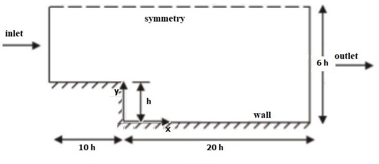
The Reynolds number is based in step height h= 0,98 cm, U velocity = 7,72 m/s and std air 20° C conditions is adopted like in JD experimental study. At inlet velocity magnitude is prescribed normal at boundary with U= 7,72 m/s and viscosity ratio of 10 (for k-epsilon and k-omega I set the turbulence intensity to 5%). At wall no slip condition and adiabatic surface is imposed and at symmetry I set as symmetry line. 

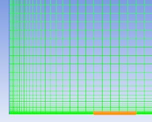
A quadrilateral structured mesh is generated with y+ < 1 in adjacent wall cells. We can see in the image below a zoomed view of mesh. 

So,Then I will demonstrate the graphs of Cf vs x / h and Cp vs x / h displaying experimental and numerical results from the Sparlat-Allmaras model.

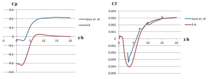
As expected we can see a double change of sine on the chart Cf vs x / h which indicates the presence of a recirculation zone composed of two bubbles, one smaller at the base of the step and one larger a little forward. This is shown by the image below with the colored vectors for velocity, results for model S-A.

The Xr indicates the reattach length and for this case we get a Xr/h value equal Xr/h = 6.5. According with the experimental data from JD the mean value of rettach length is Xr/h = 6+- 0.15. An acceptable difference of 8.33%. 

It is visible that, by plotting Cf vs x / h, the result obtained by FLUENT overpredicts the coefficient of friction experimental curve and has values closer after the reconnection zone.

But what intrigues me is because the graph of the pressure coefficient is so below the experimental one that the graph Cf vs x / h has an acceptable agreement between the curves? Is it because of this approach being 2D and the real approach being 3D? Together with the experimental material, it contains results for a 3D simulation by DNS that the values coincide for both the pressure coefficient and the skin friction coefficient. I tested severe differences between models (I only showed the result S-A because they all exhibited similar behavior), I changed pressure-velocity coupling, etc. but they all exhibited satisfactory agreement for Cf, but for Cp no? What could be behind it? This is the big question ...

Enjoy the conversation! 

Mantovani. 

[Karthik Remella]

Hi,

Very interesting results. Couple of questions / clarifications:

• Have you tested 3D simulations using various models?


• Probably you mentioned, but I wanted to still ask for further clarity - did you run other model (k-omega SST and realizable k-epsilon with enhanced wall treatment) and still get a difference in C_p?


• I am sure you must have done this, but I still want to pose this question here: Have you double-checked the values of reference pressure, velocity, and density you are using to estimate the pressure coefficient in Fluent with those from the paper? The reason why I am asking you this question is because of the nature of the two curves. It is almost like the two curves are offset by a constant number.

I hope this helps.

Thank you

Best Regards,

Karthik

[Amine Ben Hadj Ali]

Hi,

to add to Kremella important suggestions to use a more sophisticated turbulence model is to check the reference values in Fluent which are used for the calculation of skin friction and pressure coefficient.

 

A.

[José Mantovani]

As Kremella said I also thought that the curves of the Cp chart were 'compensated' by a constant and it made the difference because in the format they are very similar. But I used the same values for expression Cp, which I used in the expression Cf which in the case was satisfactorily good and very close as can be seen by the image.

I defined the Cp as -> Pressure / (0.5 * 1.225 [kg / m ^ 3] * (7.72 [m / s]) 2)

Looking at the conditions of the experiment they used 1.2 [kg / m ^ 3], which altering does not generate much difference. But in the part where the calculation of Cp is spoken I realized that it was done differently, see image below with the explanation of how it was done. (IMAGE EXTRACTED FROM JD EXPERIMENT PAPER).

Any suggetion of how Can I measure the wall static pressure at x/h=-5.1 to input in Cp expression?

Mantovani. 

[klu]

Hi Jose,

To obtain the pressure at x/h = -5.1, you might create a point from Surface -> Create at the location and then compute the area-averaged static pressure at the point using the Surface Integral in Report. 

Thanks,

Kun

[José Mantovani]

Ok, I will try this and post here the results. 

And how would my expression look for Cp by measuring this pressure at x / h = -5.1? It would look like:

Cp exp = (Pressure - Pressure at. x/h= -5.1 )/ (0.5 *1.225 [kg / m^3]*(7.72[m/s])^2)

Like this?

Thanks for attention and helping!

Mantovani. 

[klu]

Yes according to the definition in the paper. However unless the Pressure at x/h=-5.1 is negative, your Cp profile will not move upward. So please share your results after the expression is updated.

[José Mantovani]

Hello guys, So I tried to get a converged Cp chart with the experimental. I measured the wall static pressure at x/h= -5.1 and input in the expression according with the image below.

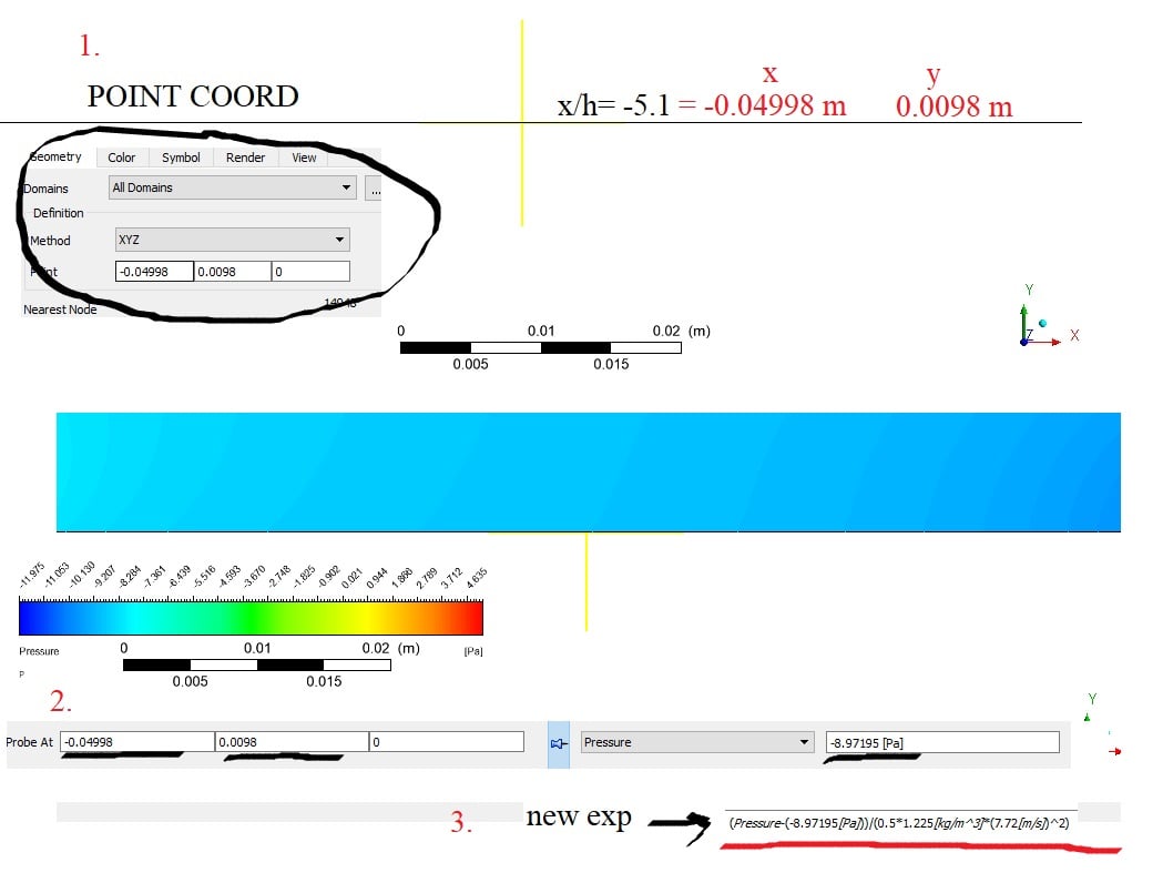
Now the Cp chart is better than before, but is still above the experimental, I will see if I improve the mesh (imposing a higher density near the step with a horizontal edge sizing and not just vertical towards the wall). But it is already better than before, for the k-epsilon and k-omega models I adopted turbulence intensity equal to 1%, according to the JD experiment the measurements indicated below 1% but it is not written exactly as it was.

Below have the vectors ploting velocity, we can see the difference of recirculation region through different turbulence models. For the S-A the reattach lenght is about 6.5h, for Real k-e and SST k-omega about 6.8h, according with JD experiment the reattach length is 6 +-0.15 h. 

The presented k-omega SST solution did not converge below the established criterion (I did last night and because of sleep I did not continue the simulation) then the SST k-omega result is not accurate. I will improve the mesh and test various configurations. But what do you think of the results? Seeing the procedure as I did, the mesh, it is always possible to get a better result, but what do you think of these? Regarding the graphics, does anyone have any hints as to why FLUENT generates a larger Cp compared to experimental data? Overpredict the Cp curve ... As we can see through the graphs and vectors images, there is a difference between the behavior of the recirculation zone through the different models tested, some generate the largest minor bubble, another generates the largest bubble longer ...

Thank's for helping and support guys!

Mantovani.

[José Mantovani]

Could anyone comment on the results? Any idea of why the simulated values overpredicts the experimental data?

Thanks again.

Mantovani. 

[Karthik Remella]

Hello Jose,

I think your work is extremely interesting, diligent, and through. Couple of thoughts on your results:

• Are you using a constant inlet velocity condition? Have you tried to obtain a fully developed streamwise periodic profiles for all inlet specifications and use these profiles to run your simulation?


• What are your Turbulence specifications in your velocity inlet BC? Have you tried changing them?


• What about generating a tighter mesh in the horizontal direction (especially near the step)?


• What is your growth rate for your current mesh?

These are some really broad thoughts I have at this point. Hope this helps.

Best Regards,

Karthik

[José Mantovani]

Hello Kremella, I'm glad you think that of my work and helping me. I am writing an article about this to publish at a symposium that occurs annually in my college and what is missing is just the results and discussion section. Regarding your tips I will talk about them:

1. Yes, I am using uniform velocity profile at the inlet, for that in another publication an ANSYS engineer told me to use it as long as the length of the input duct is long enough to develop the flow.

2. For the turbulence specifications at the inlet I used a viscosity ratio of 10 and a turbulence intensity of 1%, due to the JD experiment the turbulence intensity value measured in the wind tunnel was below 1%.

3. I actually generated a mesh in this way, tightened in the horizontal direction (increasing the density near the step), but I had extreme difficulty converging the results even in the model of an S-A equation. FLUENT accused reverse flow and it took a long time for the iterations to be calculated and more to converge, I used the Coupled scheme for pressure-velocity coupling and solved (this numerical procedure for those models that presented the above results) using the first interpolation order upwind until converging to a normalized error factor of 10 ^ -3, then changed the interpolation scheme to second order and the factor to 10 ^ -6 by calculating until convergence (I used standart initialization computing by inlet). Maybe for this tight mesh in the horizontal direction I should use another coupling and interpolation scheme, can you tell me how to perform numeric procedure for this type of mesh? Maybe QUICK interpolation scheme since the mesh is quadrilateral structured, I do not know... I also have difficulties to converge the solution using the Std. k-epsilon (being that for Realizable k-epsilon it's easy and fast), more night I'm going to test the RNG k-epsilon model and the Std. k-omega. I dont know if I should use different numerical procedure for each mode, I dont know, really the Std k-epsilon model is very difficult to obtain convergence for this current mesh.

4. The growth rate for my current mesh is default. 

Thank you immensely for your help Kremella and look forward to your return post. I will wait to see how I should proceed so that I can finish my work.

Mantovani.

 

[Karthik Remella]

Hello Jose,

Firstly not all models give you the same level of accuracy. Some model are more accurate than others and the accuracy is dependent on the physics of the problem. Having said that, you seem to be using the right models to solve this problem. The curious part about your results is that the discrepancy (over-prediction) seems to be occurring even before the step (~ 6h - 7h region). Can you try to refine the grid in the upstream area of the step? 

If you have a sufficiently long upstream channel to allow the flow to become developed, you are fine. You do not have to run the stream-wise periodic simulation. Again, whether you want to use a fully developed profile or not is also dependent on the conducted experiment. How different is your geometry from the conducted experiment?

If you haven't already tried, please give 'Turbulence intensity and hydraulic diameter' a shot. You should be able to change this from the boundary conditions panel - inlet velocity and pressure outlet.

If you are running a steady state model, perhaps you could try using 'pseudo-transient' settings?

Dumb question - are your simulation results mesh independent?

Thank you.

Best Regards,

Karthik

[José Mantovani]

Hello Kremella, read item 3. again, I edit it now.

Thanks.

[José Mantovani]

 

Hello, so Kremella you say to me try to create a tighter mesh in horizontal direction and I found a pdf archieve of some validation cases in internet using FLUENT. In image below have the section about the BFS simulation with comments over mesh, numerical procedure and Cf graph results and in this case the autor used a tighter mesh in horizontal direction and the results is very similar with my results... Look. He also used 10h of inlet duct length and uniform velocity profile at inlet boundary. 

If we compare these graphs with those that I get the over-prediction is smaller, because mine has minimum values of -0.004 while in that it obtained values of -0.006 ... I wanted to understand why this variation occurs because the FLUENT over-predict the experimental result, seeing these results I think that mine is good enough ... But how stubborn I think I can improve and I keep trying.

Mantovani. 

[Karthik Remella]

Hello Jose,

Thank you for sharing these materials here. These would be extremely useful resources for someone who is looking for some literature on this problem.

To answer your question: it is extremely hard to me to explain why Fluent model (in the above post) shows different results from yours without taking a deeper look into the two models. Without a side-by-side comparison, all I can do is surmise. However, I will leave you with one thought here. All turbulence models are not equally accurate when it comes to their applicability to different problem. They, within reason, predict the physics and their applicability is dependent on the nature of physics. Each turbulence model has inherent approximations and simplifications (which are made to make the numerical problem tractable). On one hand, these approximations allow us to solve the model and make the problem more tractable computationally. While on the other hand, they sometimes show deviations from the actual physics. Another note: when comparing the model and results from experiments, it is extremely important to maintain consistency and question all assumptions (both from model as well as experiments). I am not sure if this is very helpful with matching your results.

I still believe we are missing something simple. It might not be your model set-up. Perhaps you should give grid refinement (in the bulk regions of your flow) a shot. Perhaps, you want to attach your simulation files and have someone look at them (just to engage a new pair of eyes)?

Thank you.

Best Regards,

Karthik

[brbell]

I just saw this discussion yesterday. I have previously done studies of backward facing step flow from Vogel & Eaton (1985) and also Driver & Seegmiller (1985), so I would like to make an observation.

Results downstream of the step are very sensitive to the boundary layer profile at the step.  In both the cases mentioned above, as well as the Driver & Jovic case, experimental measurements are reported at a location a few step heights upstream of the step.  The boundary layer in the CFD simulation should match the experiment at this location or else agreement with measurements downstream of the step will suffer.  

In particular, the boundary layer thickness, displacement thickness and momentum thickness in the CFD boundary layer should be reasonably close to the experimentally reported values, or at a minimum, the boundary layer thickness should be the same. The flow in these experiments is a zero pressure gradient flat plate boundary layer flow with boundary layer thickness ~1.2h at the step, not a fully developed duct flow where the boundary layer thickness would be 1/2 of the channel width (that would be 5h here).  (edit: corrected error in channel width)

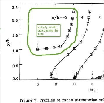
The attached picture shows the velocity profile from the experiment at x=-3h  (and the numerical values are in the appendix).  Wherever the inlet of the computational domain is located, whether -6h, -10h, -20h, ..., if the velocity profile in the simulation does not look like this at x=-3h, comparison with experimental measurements will be difficult.

I prefer to do an auxiliary calculation of the upstream wind tunnel section to generate a profile with the same boundary layer thickness and free stream velocity as the experiment.  This also has the advantage of providing profiles of the turbulence model variables.  This is just a personal preference and other methods may be possible.

One final observation is that Re=5100 is a low Reynolds number for a turbulent flow.  As a consequence, I would not expect any of the k-epsilon models with enhanced wall treatment to work very well because it is likely that large regions of the domain, even outside of the boundary layer, will be in the viscosity affected region (Re_y < 200, see the documentation) where epsilon is prescribed rather than computed. It is problematic for separated flow when the EWT viscosity affected region extends outside of the boundary layer.  

[José Mantovani]

Oh my God Br Bell, this helping is very very powerful. Keep helping me like this.

So I really thought about this question of the thickness of the boundary layer, the thickness of the momentum and the displacement of the boundary layer really should present agreement otherwise we will get the results that I actually obtained. But how could I configure this? Maybe this is the missing point ...

I would like to know how I can do this because I do not know, you mentioned the measurement that I had already visualized (velocity profile at x / h = -3), how can I model it?

You also said about height 5h, in the schematic view I put of the computational domain at the beginning of the thread the maximum height is 6h should it be corrected for 5h? (is that it? I don't understand if the 6h dimension is correct or wrong).

How could I do this auxiliary calculation? Can you give me more detail on how to proceed?

And with regard to the final observation, in my work I had the idea of evaluating all the models including indicating the best and the worst for this since each one has a purpose through the restrictions and simplifications contained, as Kremella explained, but through his final observation which model would be the best for such?

Really really really thanks! I'm waiting for answers!

Mantovani. 

[brbell]

Hi Mantovani,

To generate inlet profiles, I create an auxiliary domain consisting of the upstream section of the wind tunnel, designated by the blue line in the picture.  

Here I would probably just go from inlet at -(38.4 + 7.6) to outlet at 0.  The streamwise grid spacing at the inlet should be small and it can expand downstream, something like the picture below. 

Velocity profile at the inlet is uniform, turbulent intensity and viscosity ratio 0.1 & 1.  You don't know what the velocity is at the inlet of the wind tunnel, only at the reference location so start with the Uo reported in the paper, and then adjust it until the free stream velocity has the reported value at the reference station 3cm upstream of the step.   When it matches, compare the velocity profile with the experiment.  I would create a line at the location of the reference station and write the velocity on the line, then use Excel to compute displacement and momentum thickness.  

Hopefully there will be a good match.  In case it is not a good match, this is just an approximation of the experiment because the boundary layer was tripped and also the sidewalls of the wind tunnel diverge slightly to ensure zero pressure gradient.  If it does not match, for instance the freestream velocity matches but the boundary layer thickness does not, then you can try things like modify the intensity and viscosity ratio at the inlet, add wall roughness on a small portion near the inlet (to act like a trip) or I have even added cell zones (orange in the picture) to add a source term for turbulent kinetic energy.  Basically it is trial and error until the velocity profile has reasonable agreement with the experiment.  Then I write the profile and use it as the inlet.  

The height of the test section upstream of the step should be 5h.  In the schematic, the outlet is shown as 6h, which is correct because the expansion due to the step is 1.2.

I would expect k-omega models to give the best results for this case (due to low Re), but I have not actually seen a study of this problem with turbulence model comparison so it is only a guess.

 

[José Mantovani]

It's very good Br Bell, so by the thinking over the velocity profile I get this for my Realizable k-epsilon solution, which is the "best" or the most "close" result compared with the experimental data from Jovic and Driver experiment. Take a look. In image below we can see the Cf and Cp chart for the experimental and RKE solution by FLUENT. 

The values are close to reconnection, after that as you can see in the Cp chart there is an over-predict of the solution by FLUENT compared to the experimental data. So, we can take a look over the velocity profiles by the image below.

As we can see in the first chart we have the measure in the x/h= -3. If we compare with the JD measure at same location, using the image which Br Bell demostrate in image below, we can see a little difference between the JD and my solution. 

So thinking about the velocity profile, I see in the Le et. Al (1997) work, this is a Direct Numerical Simulation of this experiment. In this paper we have a section about the boundary condition, I get a image of this as we can see below. 

So, through this explanation I search by this paper of Spalart boundary layer simulation. The Le et. Al has used this as velocity profile and your results is very close with the experimental. I believe it's more or less the same path as you indicated Br Bell, calculate an auxiliary stream to get the velocity profile. So, if he used this from Spalart's work and the result was very close, I believe that if I do the same I can get something similar, since due to 2D simulation it will be difficult to recreate the zero gradient pressure boundary layer situation since here there are no side walls of the tunnel, which actually diverge to ensure this. In image below we have the results by Le et. Al using the velocity profile obtained in the way like the Spalart work, the results is very close to the experimental. I used 10h of inlet duct length due to the work of Le et. When recommending this for recovery of the turbulence characteristics of the entrance.

A little comment between my Cf chart and Cf chart in image above (of Le et. Al result) my results it's not that different or so divergent, but the problem is seen in the Cp chart where my result over-predict the experimental curve. 

So taking a quick look at this Spalart work, posted on NASA sites (https://ntrs.nasa.gov/archive/nasa/casi.ntrs.nasa.gov/19870008597.pdf) I found this image below with the spatially-developing of the boundary layer that at the beginning has a shape similar to my measurement for x / h = -3 obtained through the simulation using RKE, image below.

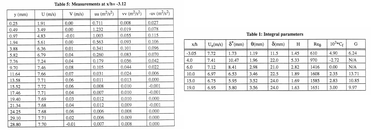
From what I understand, they used the right profile in the image, the final profile of the boundary layer as value for x / h = -3. In the JD paper also have a DNS simulation of this problem, and he also used this way to take the velocity profile. In image below, by the JD paper I found some information over the x/h= -3.12  region and integral parameters for x/h= -3.05.

So, I wanted an opinion from you Br Bell, Kremella and someone else who can help. Following what Br Bell has proposed, I believe that by trial and error this would be a bit tiring and perhaps would not get such a value.

The opinion would be about: what would be better, from the values in the picture above would I get the approximate velocity profile? Or if I replicate the Spalart simulation to use the velocity profile as the JD experiment itself used in the DNS simulation and the work of Le et. Al, too, might be closer. Or, if I use some program to collect the data from the points in the image that Br Bell extracted from the velocity profile at x / h = -3 could this possibly be used? (which I believe would be the easiest option).

In your opinion, can you give me some comment about the graphics that I put here of my solution in FLUENT? And which way do you think you can be smarter, in order to get a close result and generate the least amount of confusion (I say overwork for a bad result)?

Sirs, I am really dedicating myself to this work, because I believe that I am in fact understanding not only the functioning of the software but also because of the incessant search for the good result, I am better understanding how the flow works and forcing it to use different methods, UDF for velocity profile, something I've never used and I believe I'll have to use that case. I hope to count on your help and I await an answer.

Really thanks for the attention, I'm doing my best in this job and will only stop when I actually finish.

Mantovani. 

[José Mantovani]

Here we have the image extracted from Le et. Al work of the velocity profiles. For comparasion with my velocity profiles obtained by FLUENT solution using RKE.

 

[brbell]

Hi Mantovani,

Measured values for the velocity profile at x/h = -3.12 can be found in the appendix, Table 5, of the Jovic and Driver paper, which you included in your post.  There is no need to measure these off the plot in my post from yesterday.  I suspect in the plot legend they just rounded -3.12 to -3 for display.

Similarly, measured values at other locations downstream of the steps can be taken from tables in the appendix and used for plotting against the CFD results.

I would expect the velocity profile from the Spalart DNS would work here too, as Le et al. obtained good results while using it.  The Spalart profile data is available in the ERCOFTAC database, which I will link in just a minute (scroll down in the .dat file to find the values from Re_theta = 670)

 http://cfd.mace.manchester.ac.uk/ercoftac/database/cases/case33/Case_data/

 Profiles from the Le and Moin DNS can also be obtained from the ERCOFTAC database

http://cfd.mace.manchester.ac.uk/cgi-bin/cfddb/prpage.cgi?31&DNS&database/cases/case31/Case_data&database/cases/case31&cas31_head.html&cas31_desc.html&cas31_meth.html&cas31_data.html&cas31_refs.html&cas31_rsol.html&1&0&0&0&0

I would feel comfortable using their x/h = -3 values as the BC for RANS, and they also include the tke profile

 Finally, sorry for so many edits, the website is not processing when I hit post.  

Using a profile to define the boundary conditions will probably be easier than a UDF.  It is just a simple text file with velocity (and any other variables) as a function of position.  The help section on using profiles has information on how to create and use them

 https://ansyshelp.ansys.com/account/secured?returnurl=/Views/Secured/corp/v190/flu_ug/flu_ug_sec_bc_prof.html

[José Mantovani]

It's very good Br Bell, really thanks for your help. I will try in some ways and I will inform as much as I can. 

I will try use the velocity profile of link which you put above. 

Just to see if I understand, when you say that you would feel comfortable using the profile I measured at x / h = -3, you mean to use that profile in the inlet of my computational domain? Together with TKE ... 

For the time being I understand, I'll try this, and those available on the CFD ERCOFTAC website of the Le & Moin study.

Answer me when you can, just to confirm if that's what I understood. I will try all the possibilities and soon I will make available the results obtained here. Thank you very much and heartily of your help and of all, really thank you.

Have a very nice friday night!

Mantovani. 

[brbell]

Hi Mantovani,

In my post, I meant I would be comfortable using this velocity profile as a boundary condition at the inlet of the computational domain:

I think the first few points of this table are what is plotted in Figure 7 of the Jovic and Driver paper.  They only report and .  To get tke,   is also required. Maybe it can be estimated.   Anyway, in addition to using a realistic, non-uniform velocity profile as the inlet boundary condition for the computational domain, it is normally also useful to also have matching non-uniform profiles for the turbulence model variables.  The turbulence model information is readily available from a precursor calculation, but would need to be estimated somehow from whatever experimental data is available.

[José Mantovani]

Very thanks Br Bell! I will try using this values of Table 5 with estimated w'w' and the values of Le and Moin archieve. 

In a few days I share with you the results I obtained from the two velocity profiles. I'm going try to use the profile method because UDF does not know how to use it and seems to be more difficult than profile method. 

I will look in the user guide FLUENT how to impute this profile as a boundary condition (at inlet), if I can not I will ask again here, by the hour thank you for the attention and help. Very soon I share my results here.

Thanks one more time,

Mantovani. 

[José Mantovani]

So guys, in recent days I had to pay attention to other projects of mine and still could not create the velocity profile according to above.

But, as can be seen in the course of the discussion the graphs of Cf vs x/h and Cp vs x/h exhibits a good agreement, for Cf vs x/h in view of the differences and 2D approach in my opinion is very satisfactory, the graph Cp vs x/h shows a behavior very close to the end of the recirculation zone where the flow reconnects and the graph of Cp begins to diverge.

How can I to interpret this? Merely a coarse mesh in region? Can anyone comment on the Cp chart? What could cause the divergence there? If the velocity profile at the inlet is not exactly the same as the experiment and yet the graph exhibits a similar behavior, why does it begin to diverge at the point of reconnection?

Can anyone help me to interpret this? Any guess? 

As I am not having time to do the velocity profile file and even without it the graphics present good agreement I am thinking of finalizing the article with an explanation for the divergence of the graph Cp vs x / h while testing other meshes in order to check if I get a better result.

Thanks for helping and support!

[brbell]

Hi Mantovani,

According to results in this paper (sorry it is not fulltext but maybe available through your library resources),

https://arc.aiaa.org/doi/abs/10.2514/6.2003-765

It is possible to simulate this low Re backstep, with Fluent, and closely match the experimental Cp values.   

So there must be some difference between what you are doing and what the authors of the paper did.  

Without investigating the sensitivity of the results to the inlet profile, and the sensitivity to systematic grid refinement, it might be hard to understand the Cp results.  For finalizing the article, I would be inclined to say that the divergence in the graph of Cp is probably due to uncertainty in the boundary conditions.

 

 

[José Mantovani]

Hello Br Bell. 

Sorry for the delay in responding because I tried to extend the domain after the step to see if the result of Cp improved. What happened was that the Cp result remained the same, there was a slight difference in the reconnection length that reached values within the experiment between 6 + -0.15.

I would like to try to do a mesh indepedence study because I still have a few days to send this work, can you give me tips on how to proceed? 

The graph of Cf vs xh presented a good result (comparing with that of Le and Moin's work was very close) only the graph of Cp even though it had this variation, perhaps due in the experiment the walls of the tunnel had slight divergence to guarantee a gradient zero pressure or else may be due to the same inlet conditions or due the mesh as you said... 

I took a look at the ERCOFTAC database and I think that here in this link I have the conditions of inlet into physical dimensions, could you take a look and confirm? The one where you told me that in the case is the same, but directly from the study of Spalart is y+ u+ dimensions. 

http://cfd.mace.manchester.ac.uk/ercoftac/database/cases/case31/Case_data/x.181

In the file read me have the explanation about the names of file and for 181 is the x/h= -3. Can I use this file as inlet condition? I think this stay in physical dimensions, can you take a look in way to confirm this?

Very thanks for your support and helping dear friend Br Bell. 

Mantovani. 

[brbell]

Hi Mantovani,

The normal way to do a mesh independence study would be to double the number of grid points in all directions.  If that is not viable because it would result in too many cells in the mesh, increase the number of grid points by some factor smaller than 2.  After converging the solution, compare it with the solution from the original grid.  It is probably a good idea to be careful on judging convergence.  Sometimes the solution might still be changing even though the residuals have all reached .001

The reference linked in my previous post shows that good agreement with Cp is possible.  It is hard guess why you are getting the overshoot in your Cp plot.

I looked at the readme file from the cfd.mace.manchester.ac.uk link.  It says the velocity is normalized by the freestream velocity and y by the step height, so the values are not u+ and y+ but they are still dimensionless.  The fluctuating velocities are also normalized by the freestream velocity.  I think the freestream velocity is known so converting to physical dimensions is just a simple multiplication.

[José Mantovani]

Hello Br Bell.

I understood. I tried in this way but the values that I get is very close with the results which I get before. I saw the paper that you sent and really the results stay very close. I tried in many ways really do not know what happens, I use a thick mesh ("2D surface mesh"), I tried to use with 1 cell thick but nothing has changed.

I found this file of the velocity profile less complicated because I do not have to make so many changes and the chances of making mistakes in the middle of the way is big, now with that just just multiply by velocity as you said. 

I'm going to take some time to set up this profile, I believe that some doubts appear and I'm still sharing here, if I can, I'll directly share the results here. 

I still count on your help, from time to time look here. Maybe tomorrow I'll post something here about whether or not I got the profile, some possible doubts.

Very thanks for support and helping.

Mantovani.