
-
-
July 18, 2018 at 11:57 pm
Kellen.traxel
Subscriber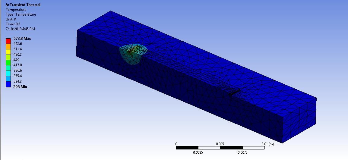
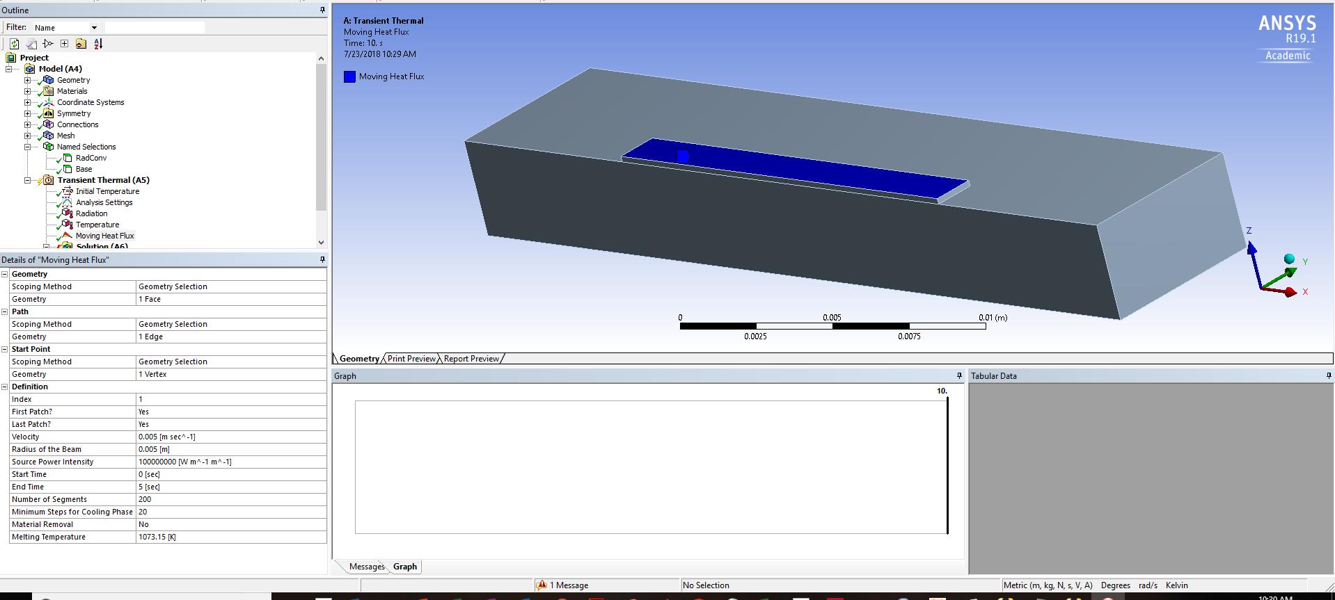
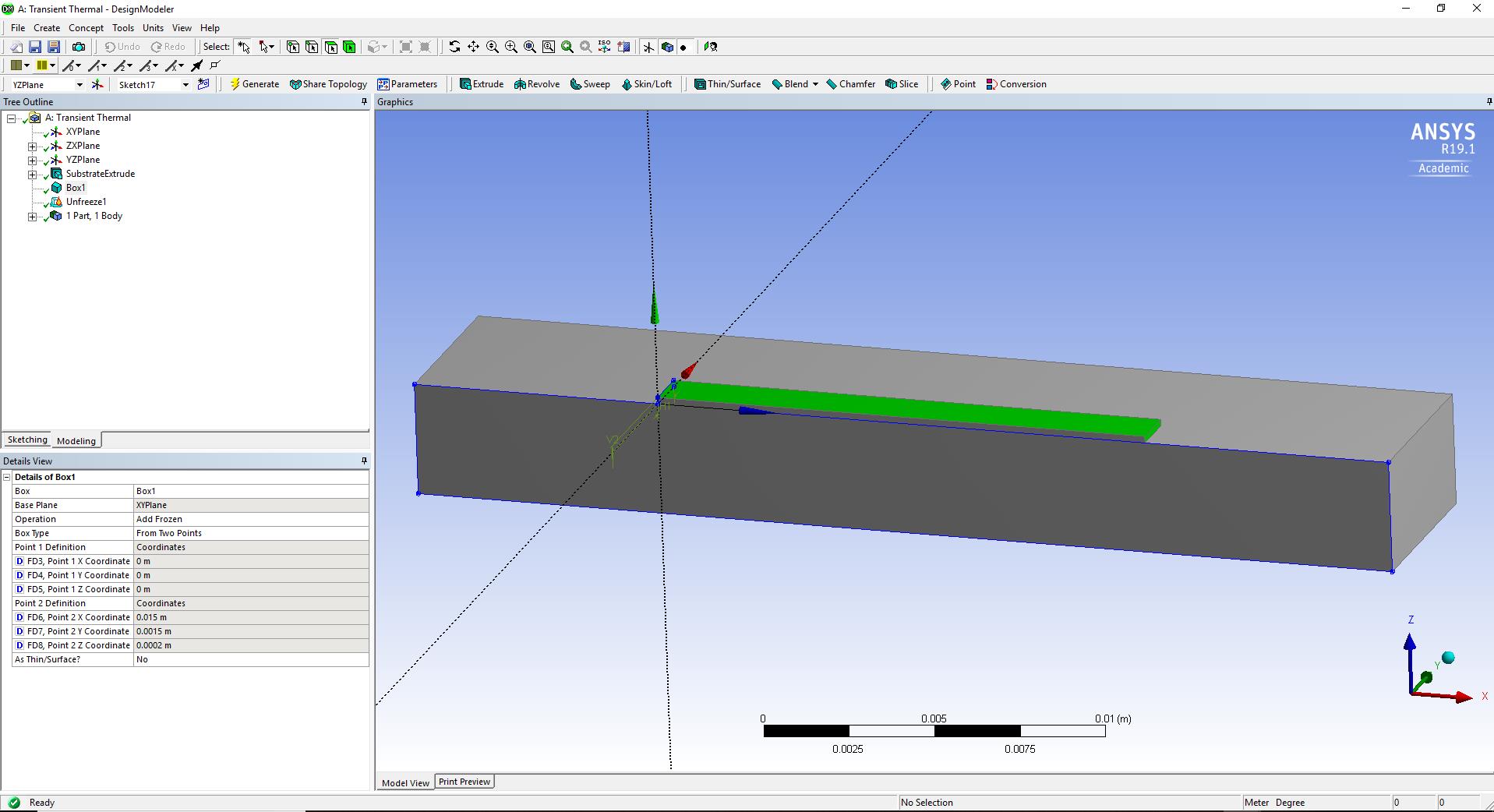
What is the most efficient way to model the laser heat source moving across my symmetric, 3D, single-layer track? I have read about using commands in APDL, however, it is not clear how I can manipulate a nodal (or volume) heat source as a function of the simulation time and position. In the image above, I was able to model a nodal heat source at the starting location (t=0) using APDL commands in the "Transient Thermal" section of my model tree. Ultimately, my question is about the relation between the APDL commands in workbench (and their location in the model tree) and the actual simulation time, and how they could be combined using a DOWHILE loop of some sort so that the local laser coordinates can translate with respect to the overall model domain. I currently do not have access to the ACT toolbox or AdditivePrint in my ANSYS Mechanical license.
Thanks in advance for any information or resources.
Regards,
Kellen
-
July 19, 2018 at 4:09 pm
jpasquerell
Ansys EmployeeSee help/ans_the/Hlp_G_THE2_9.html for an example of a 1 D tabular load. you will need a 2d table for time and a spatial coordinate variation.
-
July 19, 2018 at 4:14 pm
Sandeep Medikonda
Ansys EmployeeHi Kellen,
In general, we have an ACT extension (Moving Heat Source v4.1) that does this in the app store which would be the easiest way to go about this. Now the 1-D example that jpasquerell refers to is shown below and in your case, you would need to extend this to a 2d table which includes both time and coordinate variation.
/batch,list
/show
/title, Demonstration of position-varying film coefficient using Tabular BC's.
/com
/com * ------------------------------------------------------------------
/com * Table Support of boundary conditions
/com *
/com * Boundary Condition Type Primary Variables Independent Parameters
/com * ----------------------- ----------------- ----------------------
/com * Convection:Film Coefficient X -
/com *
/com * Problem description
/com *
/com * A static Heat Transfer problem. A 2 x 1 rectangular plate is
/com * subjected to temperature constraint at one of its end, while the
/com * remaining perimeter of the plate is subjected to a convection boundary
/com * condition. The film coefficient is a function of X-position and is described
/com * by a parametric table 'cnvtab'.
/com **
*dim,cnvtab,table,5,,,x ! table definition.
cnvtab(1,0) = 0.0,0.50,1.0,1.50,2.0 ! Variable name, Var1 = 'X'
cnvtab(1,1) = 20.0,30.0,50.0,80.0,120.0
/prep7
esize,0.5
et,1,55
rect,0,2,0,1
amesh,1
MP,KXX,,1.0
MP,DENS,,10.0
MP,C,,100.0
lsel,s,loc,x,0
dl,all,,temp,100
alls
lsel,u,loc,x,0
nsll,s,1
sf,all,conv,%cnvtab%,20
alls
/psf,conv,hcoef,2 ! show convection bc.
/pnum,tabn,on ! show table names
nplot
fini
/solu
anty,static
kbc,1
nsubst,1
time,60
tunif,50
outres,all,all
solve
finish
/post1
set,last
sflist,all ! Numerical values of convection bc's
/pnum,tabn,off ! turn off table name
/psf,conv,hcoef,2 ! show convection bc.
/pnum,sval,1 ! show numerical values of table bc's
eplot! convection at t=60 sec.
plns,temp
fini
-
July 22, 2018 at 8:31 pmSubscriber
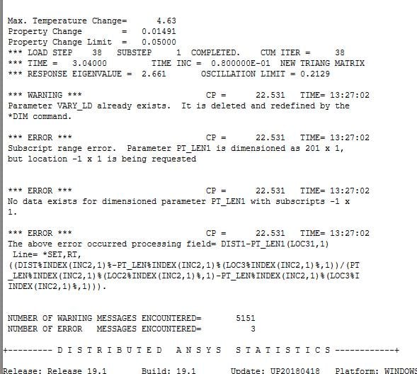
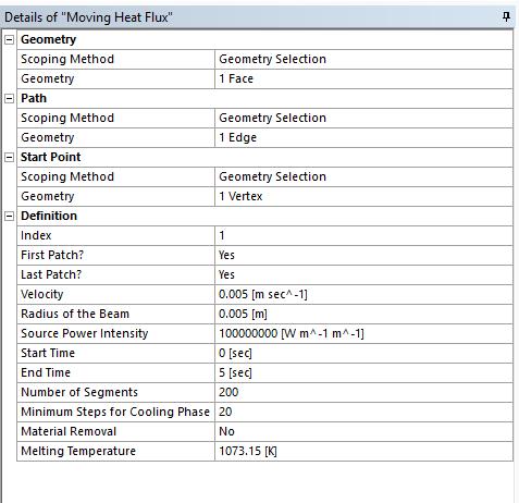
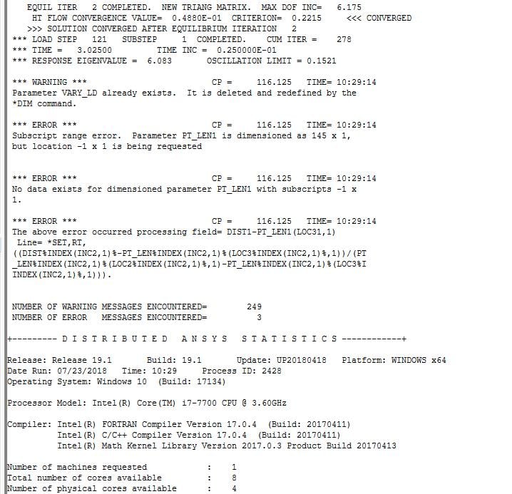
Thanks Sandeep. I just got access to the ACT so I have been trying to use the Moving Heat Source extension (I am running ANSYS 19.1). I keep running into issues in the provided code such as that shown in the attached image (from the solution information output). I am using some of the main input parameters for the moving heat source, so I am wondering if you have any suggestions for working with the plugin, or if there is a much depeer issue going on. Perhaps you might have some strategies or best practices for debugging issues such as these. Seems like there are lots of "warnings" that occur when using this plugin.
Warm regards,
Kellen
-
July 22, 2018 at 8:43 pmAnsys Employee
Kellen,
The ACT extension does mention that it supports version 17.0, 17.1 and 17.2. I believe that this could be the problem.
I will reach out and see if there is a solution to fix this.
Regards,
Sandeep
-
July 23, 2018 at 4:26 pmAnsys Employee
Hello Kellen,
I've just confirmed that the error is nothing to do with an incompatible version of ACT extension. This act extension also contains source code so you can load it in any ANSYS version without any issue. Now, regarding this error, try to check the max end time on the last moving heat definition is more than 'Path length/Velocity'. It could be the highest next whole integer and make sure 'Step End Time' under Analysis setting is more than the highest 'End Time' defined in 'Moving heat flux'.
Let me know if that helped?
~Sandeep
-
July 23, 2018 at 5:06 pmSubscriber
Hi Sandeep, I believe I had the proper settings for the heat source (See attached output information). I get a few warning messages but no errors, however, I get an error message that occurs during running and then there is no output.
Solver Output
ANSYS Academic Research Mechanical
*------------------------------------------------------------------*
| |
| W E L C O M E T O T H E A N S Y S (R) P R O G R A M |
| |
*------------------------------------------------------------------*
***************************************************************
* ANSYS Release 19.1 LEGAL NOTICES *
***************************************************************
* *
* Copyright 1971-2018 ANSYS, Inc. All rights reserved. *
* Unauthorized use, distribution or duplication is *
* prohibited. *
* *
* Ansys is a registered trademark of ANSYS, Inc. or its *
* subsidiaries in the United States or other countries. *
* See the ANSYS, Inc. online documentation or the ANSYS, Inc. *
* documentation CD or online help for the complete Legal *
* Notice. *
* *
***************************************************************
* *
* THIS ANSYS SOFTWARE PRODUCT AND PROGRAM DOCUMENTATION *
* INCLUDE TRADE SECRETS AND CONFIDENTIAL AND PROPRIETARY *
* PRODUCTS OF ANSYS, INC., ITS SUBSIDIARIES, OR LICENSORS. *
* The software products and documentation are furnished by *
* ANSYS, Inc. or its subsidiaries under a software license *
* agreement that contains provisions concerning *
* non-disclosure, copying, length and nature of use, *
* compliance with exporting laws, warranties, disclaimers, *
* limitations of liability, and remedies, and other *
* provisions. The software products and documentation may be *
* used, disclosed, transferred, or copied only in accordance *
* with the terms and conditions of that software license *
* agreement. *
* *
* ANSYS, Inc. is a UL registered *
* ISO 9001:2008 company. *
* *
***************************************************************
* *
* This product is subject to U.S. laws governing export and *
* re-export. *
* *
* For U.S. Government users, except as specifically granted *
* by the ANSYS, Inc. software license agreement, the use, *
* duplication, or disclosure by the United States Government *
* is subject to restrictions stated in the ANSYS, Inc. *
* software license agreement and FAR 12.212 (for non-DOD *
* licenses). *
* *
***************************************************************
Release 19.1
Point Releases and Patches installed:
ANSYS, Inc. Products Release 19.1
SpaceClaim Release 19.1
CFX (includes CFD-Post) Release 19.1
Chemkin Release 19.1
EnSight Release 19.1
FENSAP-ICE Release 19.1
Fluent (includes CFD-Post) Release 19.1
Forte Release 19.1
Polyflow (includes CFD-Post) Release 19.1
TurboGrid Release 19.1
Aqwa Release 19.1
Customization Files for User Programmable Features Release 19.1
Mechanical Products Release 19.1
Icepak (includes CFD-Post) Release 19.1
Remote Solve Manager Standalone Services Release 19.1
Creo Elements/Direct Modeling Geometry Interface Release 19.1
Creo Parametric Geometry Interface Release 19.1
SOLIDWORKS Geometry Interface Release 19.1
ANSYS, Inc. License Manager Release 19.1
***** ANSYS COMMAND LINE ARGUMENTS *****
BATCH MODE REQUESTED (-b) = NOLIST
INPUT FILE COPY MODE (-c) = COPY
DISTRIBUTED MEMORY PARALLEL REQUESTED
2 PARALLEL PROCESSES REQUESTED WITH SINGLE THREAD PER PROCESS
TOTAL OF 2 CORES REQUESTED
DESIGNXPLORER REQUESTED
MPI OPTION = INTELMPI
INPUT FILE NAME = C:MODELING_@SchoolBimetallic AM @ SchoolTi6Al4V-IN718ANSYSTitanium 3D Single Layer_ProjectScratchScrF1EAdummy.dat
OUTPUT FILE NAME = C:MODELING_@SchoolBimetallic AM @ SchoolTi6Al4V-IN718ANSYSTitanium 3D Single Layer_ProjectScratchScrF1EAsolve.out
START-UP FILE MODE = NOREAD
STOP FILE MODE = NOREAD
RELEASE= Release 19.1 BUILD= 19.1 UP20180418 VERSION=WINDOWS x64
CURRENT JOBNAME=file0 10:03:40 JUL 23, 2018 CP= 0.109
PARAMETER _DS_PROGRESS = 999.0000000
/INPUT FILE= ds.dat LINE= 0
*** NOTE *** CP = 0.188 TIME= 10:03:40
The /CONFIG,NOELDB command is not valid in a Distributed ANSYS
solution. Command is ignored.
*GET _WALLSTRT FROM ACTI ITEM=TIME WALL VALUE= 10.0611111
TITLE=
Ti6Al4V_3D_SingleLayer_Model1--Transient Thermal (A5)
ACT Extensions:
MovingHeat, 4.0
dc7b91d1-0fd6-439f-811e-316ced903703, wbex
/COM, AdditiveWizard, 3.0
d670da30-b684-4a76-8cae-363c855c1121, wbex
/COM, MechanicalDropTest, 2.0
f0fd899f-9d88-4f46-8cf1-36bf5c218d65, wbex
/COM, VariableLoad, 1.0
2249b080-aa00-4f29-b52e-0e1ed5de8e1e, wbex
SET PARAMETER DIMENSIONS ON _WB_PROJECTSCRATCH_DIR
TYPE=STRI DIMENSIONS= 248 1 1
PARAMETER _WB_PROJECTSCRATCH_DIR(1) = C:MODELING_@SchoolBimetallic AM @ SchoolTi6Al4V-IN718ANSYSTitanium 3D Single Layer_ProjectScratchScrF1EA
SET PARAMETER DIMENSIONS ON _WB_SOLVERFILES_DIR
TYPE=STRI DIMENSIONS= 248 1 1
PARAMETER _WB_SOLVERFILES_DIR(1) = C:MODELING_@SchoolBimetallic AM @ SchoolTi6Al4V-IN718ANSYSTitanium 3D Single LayerTi6Al4V_3D_SingleLayer_Model1_filesdp0SYSMECH
SET PARAMETER DIMENSIONS ON _WB_USERFILES_DIR
TYPE=STRI DIMENSIONS= 248 1 1
PARAMETER _WB_USERFILES_DIR(1) = C:MODELING_@SchoolBimetallic AM @ SchoolTi6Al4V-IN718ANSYSTitanium 3D Single LayerTi6Al4V_3D_SingleLayer_Model1_filesuser_files
--- Data in consistent MKS units. See Solving Units in the help system for more
MKS UNITS SPECIFIED FOR INTERNAL
LENGTH (l) = METER (M)
MASS (M) = KILOGRAM (KG)
TIME (t) = SECOND (SEC)
TEMPERATURE (T) = CELSIUS (C)
TOFFSET = 273.0
CHARGE (Q) = COULOMB
FORCE (f) = NEWTON (N) (KG-M/SEC2)
HEAT = JOULE (N-M)
PRESSURE = PASCAL (NEWTON/M**2)
ENERGY (W) = JOULE (N-M)
POWER (P) = WATT (N-M/SEC)
CURRENT (i) = AMPERE (COULOMBS/SEC)
CAPACITANCE (C) = FARAD
INDUCTANCE (L) = HENRY
MAGNETIC FLUX = WEBER
RESISTANCE (R) = OHM
ELECTRIC POTENTIAL = VOLT
INPUT UNITS ARE ALSO SET TO MKS
*** ANSYS - ENGINEERING ANALYSIS SYSTEM RELEASE Release 19.1 19.1 ***
DISTRIBUTED ANSYS Academic Research Mechanical
00433995 VERSION=WINDOWS x64 10:03:40 JUL 23, 2018 CP= 0.188
Ti6Al4V_3D_SingleLayer_Model1--Transient Thermal (A5)
***** ANSYS ANALYSIS DEFINITION (PREP7) *****
*********** Nodes for the whole assembly ***********
*********** Elements for Body 1 "Solid" ***********
*********** Elements for Body 2 "Solid" ***********
*********** Send User Defined Coordinate System(s) ***********
*********** Send Materials ***********
*********** Create Contact "Contact Region" ***********
Real Constant Set For Above Contact Is 4 & 3
*********** Send Named Selection as Node Component ***********
*********** Send Named Selection as Node Component ***********
*********** Define Temperature Constraint ***********
*********** Create "ToAmbient" Radiation ***********
***************** Define Uniform Initial temperature ***************
***** ROUTINE COMPLETED ***** CP = 0.312
--- Number of total nodes = 23244
--- Number of contact elements = 4518
--- Number of spring elements = 0
--- Number of bearing elements = 0
--- Number of solid elements = 7369
--- Number of condensed parts = 0
--- Number of total elements = 11887
*GET _WALLBSOL FROM ACTI ITEM=TIME WALL VALUE= 10.0611111
****************************************************************************
************************* SOLUTION ********************************
****************************************************************************
***** ANSYS SOLUTION ROUTINE *****
PERFORM A TRANSIENT ANALYSIS
THIS WILL BE A NEW ANALYSIS
STEP BOUNDARY CONDITION KEY= 1
CONTACT INFORMATION PRINTOUT LEVEL 1
DO NOT SAVE ANY RESTART FILES AT ALL
DO NOT COMBINE ELEMENT MATRIX FILES (.emat) AFTER DISTRIBUTED PARALLEL SOLUTION
DO NOT COMBINE ELEMENT SAVE DATA FILES (.esav) AFTER DISTRIBUTED PARALLEL SOLUTION
Use Full Nonlinear Thermal Transient Solution
NLHIST: ADDED NODAL RESULTS HISTORY FOR:
NAME = MAX_TEMP
ITEM/COMP = TEMPMAX
NODE = 0
NLHIST: ADDED NODAL RESULTS HISTORY FOR:
NAME = MIN_TEMP
ITEM/COMP = TEMPMIN
NODE = 0
********* Initial Time Increment Check And Fourier Modulus *********
Specified Initial Time Increment: 0.1
Estimated Increment Needed, le*le/alpha, Body 1: 0.112461
Estimated Increment Needed, le*le/alpha, Body 2: 0.00316329
****************************************************
******************* SOLVE FOR LS 1 OF 1 ****************
SPECIFIED CONSTRAINT TEMP FOR PICKED NODES
SET ACCORDING TO TABLE PARAMETER = _LOADVARI64
SPECIFIED CONSTRAINT TEMP FOR PICKED NODES
SET ACCORDING TO TABLE PARAMETER = _LOADVARI44
USE AUTOMATIC TIME STEPPING THIS LOAD STEP
USE 100 SUBSTEPS INITIALLY THIS LOAD STEP FOR ALL DEGREES OF FREEDOM
FOR AUTOMATIC TIME STEPPING:
USE 1000 SUBSTEPS AS A MAXIMUM
USE 10 SUBSTEPS AS A MINIMUM
TIME= 10.000
INCLUDE TRANSIENT EFFECTS FOR ALL DEGREES OF FREEDOM THIS LOAD STEP
ERASE THE CURRENT DATABASE OUTPUT CONTROL TABLE.
WRITE ALL ITEMS TO THE DATABASE WITH A FREQUENCY OF NONE
FOR ALL APPLICABLE ENTITIES
WRITE NSOL ITEMS TO THE DATABASE WITH A FREQUENCY OF ALL
FOR ALL APPLICABLE ENTITIES
WRITE RSOL ITEMS TO THE DATABASE WITH A FREQUENCY OF ALL
FOR ALL APPLICABLE ENTITIES
WRITE FFLU ITEMS TO THE DATABASE WITH A FREQUENCY OF ALL
FOR ALL APPLICABLE ENTITIES
PRINTOUT RESUMED BY /GOP
WRITE MISC ITEMS TO THE DATABASE WITH A FREQUENCY OF ALL
FOR THE ENTITIES DEFINED BY COMPONENT _ELMISC
CONVERGENCE ON HEAT BASED ON THE NORM OF THE N-R LOAD
WITH A TOLERANCE OF 0.1000E-02 AND A MINIMUM REFERENCE VALUE OF 0.1000E-05
USING THE L2 NORM (CHECK THE SRSS VALUE)
*********** Moving Heat Flux: Moving Heat Flux ***********
FINISH SOLUTION PROCESSING
***** ROUTINE COMPLETED ***** CP = 0.312
*** ANSYS - ENGINEERING ANALYSIS SYSTEM RELEASE Release 19.1 19.1 ***
DISTRIBUTED ANSYS Academic Research Mechanical
00433995 VERSION=WINDOWS x64 10:03:40 JUL 23, 2018 CP= 0.312
Ti6Al4V_3D_SingleLayer_Model1--Transient Thermal (A5)
***** ANSYS ANALYSIS DEFINITION (PREP7) *****
CMBLOCK read of NODE component FACE1 completed
CMBLOCK read of NODE component PATH1 completed
CMBLOCK read of NODE component START1 completed
You have already entered the general preprocessor (PREP7).
SELECT ALL ENTITIES OF TYPE= ALL AND BELOW
PARAMETER INX = 1.000000000
PARAMETER LSTP = 200.0000000
PARAMETER VEL = 0.5000000000E-02
PARAMETER SEG = 201.0000000
PARAMETER R1 = 0.5000000000E-02
PARAMETER LD = 100000000.0
PARAMETER TM_L = 5.000000000
PARAMETER TM_S = 0.000000000
PARAMETER FP = Yes
*IF FP ( = Yes ) EQ
Yes ( = Yes ) THEN
OPENED FILE= INDEX1.TXT FOR COMMAND FILE DATA
COMMAND FILE CLOSED
OPENED FILE= VELOCITY1.TXT FOR COMMAND FILE DATA
COMMAND FILE CLOSED
OPENED FILE= LSTP1.TXT FOR COMMAND FILE DATA
COMMAND FILE CLOSED
OPENED FILE= CON1.TXT FOR COMMAND FILE DATA
COMMAND FILE CLOSED
OPENED FILE= LD1.TXT FOR COMMAND FILE DATA
COMMAND FILE CLOSED
OPENED FILE= TMST1.TXT FOR COMMAND FILE DATA
COMMAND FILE CLOSED
OPENED FILE= TMLT1.TXT FOR COMMAND FILE DATA
COMMAND FILE CLOSED
*ELSEIF FP ( = Yes ) EQ
No ( = No ) THEN
*ELSE
*ENDIF
*GET ANSINTER_ FROM ACTI ITEM=INT VALUE= 0.00000000
*IF ANSINTER_ ( = 0.00000 ) NE
0 ( = 0.00000 ) THEN
*ENDIF
*** WARNING *** CP = 0.312 TIME= 10:03:40
SOLVE is not a recognized PREP7 command, abbreviation, or macro.
This command will be ignored.
*************** Write FE CONNECTORS *********
WRITE OUT CONSTRAINT EQUATIONS TO FILE= file.ce
****************************************************
*************** FINISHED SOLVE FOR LS 1 *************
*GET _WALLASOL FROM ACTI ITEM=TIME WALL VALUE= 10.0611111
***** ROUTINE COMPLETED ***** CP = 0.312
*** ANSYS - ENGINEERING ANALYSIS SYSTEM RELEASE Release 19.1 19.1 ***
DISTRIBUTED ANSYS Academic Research Mechanical
00433995 VERSION=WINDOWS x64 10:03:40 JUL 23, 2018 CP= 0.312
Ti6Al4V_3D_SingleLayer_Model1--Transient Thermal (A5)
***** ANSYS RESULTS INTERPRETATION (POST1) *****
*** NOTE *** CP = 0.312 TIME= 10:03:40
Reading results into the database (SET command) will update the current
displacement and force boundary conditions in the database with the
values from the results file for that load set. Note that any
subsequent solutions will use these values unless action is taken to
either SAVE the current values or not overwrite them (/EXIT,NOSAVE).
Set Encoding of XML File to:ISO-8859-1
Set Output of XML File to:
PARM, , , , , , , , , , , ,
, , , , , , ,
DATABASE WRITTEN ON FILE parm.xml
EXIT THE ANSYS POST1 DATABASE PROCESSOR
***** ROUTINE COMPLETED ***** CP = 0.328
PRINTOUT RESUMED BY /GOP
*GET _WALLDONE FROM ACTI ITEM=TIME WALL VALUE= 10.0611111
PARAMETER _PREPTIME = 0.000000000
PARAMETER _SOLVTIME = 0.000000000
PARAMETER _POSTTIME = 0.000000000
PARAMETER _TOTALTIM = 0.000000000
EXIT ANSYS WITHOUT SAVING DATABASE
NUMBER OF WARNING MESSAGES ENCOUNTERED= 1
NUMBER OF ERROR MESSAGES ENCOUNTERED= 0
+--------- D I S T R I B U T E D A N S Y S S T A T I S T I C S ------------+
Release: Release 19.1 Build: 19.1 Update: UP20180418 Platform: WINDOWS x64
Date Run: 07/23/2018 Time: 10:03 Process ID: 1132
Operating System: Windows 10 (Build: 17134)
Processor Model: Intel(R) Core(TM) i7-7700 CPU @ 3.60GHz
Compiler: Intel(R) FORTRAN Compiler Version 17.0.4 (Build: 20170411)
Intel(R) C/C++ Compiler Version 17.0.4 (Build: 20170411)
Intel(R) Math Kernel Library Version 2017.0.3 Product Build 20170413
Number of machines requested : 1
Total number of cores available : 8
Number of physical cores available : 4
Number of processes requested : 2
Number of threads per process requested : 1
Total number of cores requested : 2 (Distributed Memory Parallel)
MPI Type: INTELMPI
MPI Version: Intel(R) MPI Library 2017 Update 3 for Windows* OS
GPU Acceleration: Not Requested
Job Name: file0
Input File: dummy.dat
Core Machine Name Working Directory
-----------------------------------------------------
0 DESKTOP-4FPNVRM C:MODELING_@SchoolBimetallic AM @ SchoolTi6Al4V-IN718ANSYSTitanium 3D Single Layer_ProjectScratchScrF1EA
1 DESKTOP-4FPNVRM C:MODELING_@SchoolBimetallic AM @ SchoolTi6Al4V-IN718ANSYSTitanium 3D Single Layer_ProjectScratchScrF1EA
Latency time from master to core 1 = 0.837 microseconds
Communication speed from master to core 1 = 6947.75 MB/sec
Total CPU time for main thread : 0.3 seconds
Total CPU time summed for all threads : 0.3 seconds
Elapsed time spent pre-processing model (/PREP7) : 0.1 seconds
Elapsed time spent solution - preprocessing : 0.0 seconds
Elapsed time spent computing solution : 0.0 seconds
Elapsed time spent solution - postprocessing : 0.0 seconds
Elapsed time spent post-processing model (/POST1) : 0.0 seconds
Maximum total memory used : 21.0 MB
Maximum total memory allocated : 3136.0 MB
Total physical memory available : 32 GB
+------ E N D D I S T R I B U T E D A N S Y S S T A T I S T I C S -------+
*---------------------------------------------------------------------------*
| |
| DISTRIBUTED ANSYS RUN COMPLETED |
| |
|---------------------------------------------------------------------------|
| |
| Ansys Release 19.1 Build 19.1 UP20180418 WINDOWS x64 |
| |
|---------------------------------------------------------------------------|
| |
| Database Requested(-db) 1024 MB Scratch Memory Requested 1024 MB |
| Maximum Database Used 13 MB Maximum Scratch Memory Used 3 MB |
| |
|---------------------------------------------------------------------------|
| |
| CP Time (sec) = 0.344 Time = 10:03:40 |
| Elapsed Time (sec) = 2.000 Date = 07/23/2018 |
| |
*---------------------------------------------------------------------------* -
July 23, 2018 at 5:25 pmAnsys Employee
Hi Kellen,
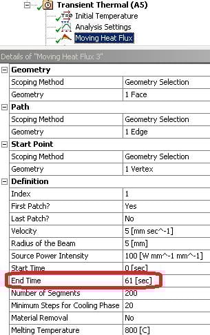
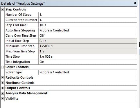
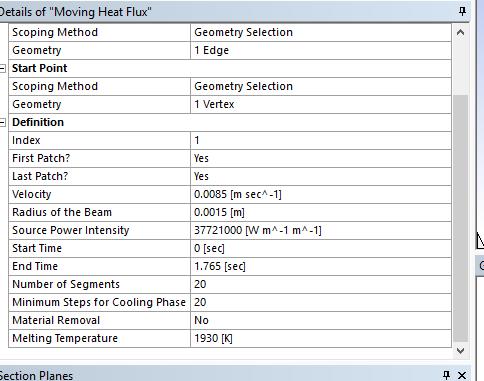
It looks like you might not have set the 'Last patch ' correctly. If there is only one moving heat load then 'first patch' and 'last patch' are both yes
If this doesn't help, can you post some snapshots of your setting and attach the complete log file?
~Sandeep
-
July 23, 2018 at 5:32 pmSubscriber
Here's some images. Not sure how to attach the complete log file, however. Let me know how to accomplish that if need be.
-
July 23, 2018 at 5:34 pmSubscriber
Still getting same issue as before. From log file:
-
July 23, 2018 at 5:50 pmAnsys Employee
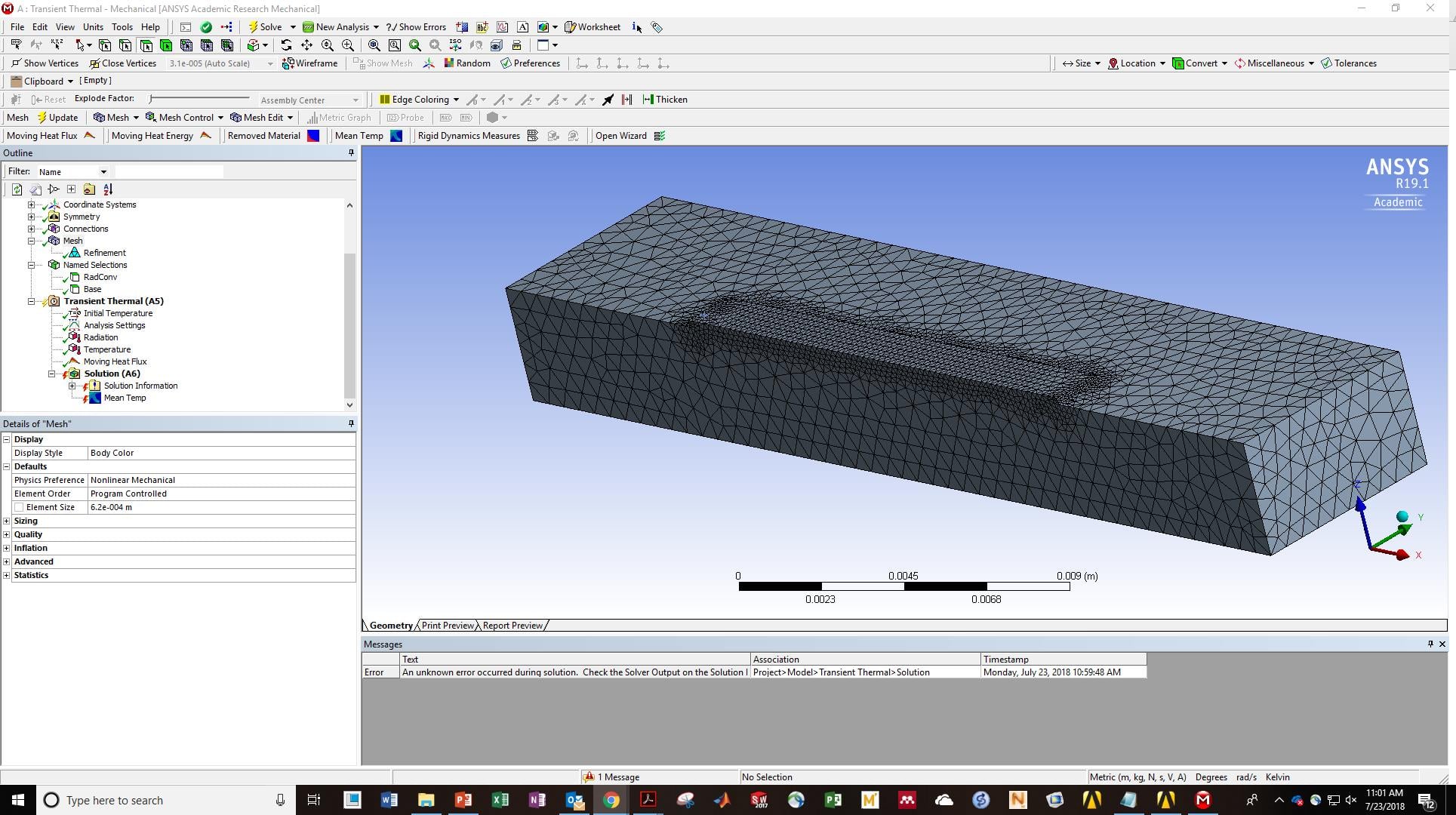
Kellen, can you post a snapshot of the length of the path (edge) and also the mesh plot?
-
July 23, 2018 at 6:03 pmSubscriber
Length of path is 0.015m
-
July 23, 2018 at 6:34 pmAnsys Employee
Kellen, Can you put 3sec as end time for moving heat source and try to solve it?
-
July 23, 2018 at 7:02 pmSubscriber
Program running now, pretty slow so I will let you know when it finishes.
Thanks
Kellen
-
July 23, 2018 at 7:38 pmAnsys Employee
Ok Awesome, The speed could be because you do have a fine mesh or it could be the machine too. To speed it up you can change the 'number of segments' but it would reduce accuracy.
-
July 23, 2018 at 8:11 pmAnsys Employee
Additionally, the reason it ran is that your End Time was way off 5 sec. Now, the path you specified is 0.015 m long and the velocity is 0.005, so it would take 3 sec. Now, in cases where it would take 2.7 sec then round it off and make it 3 seconds.
-
July 24, 2018 at 12:42 amSubscriber
Got it to run. So I basically need to make sure that my end time is close to the actual travel time? Also, does the moving heat source utilize a "quiet" or birth and death technique so that there isn't conduction through "unprinted" material?
Thanks
Kellen
-
July 24, 2018 at 11:44 amAnsys Employee
Hi Kellen,
Yes, it needs to be close to the time you are specifying in the Moving Heat Flux. I saw some EKILL commands being used in the code, so it's probably the birth-death technique. If you are interested, you should be able to access all of the APDL (+ python) code in the act extension:
~ACT_MovingHeat_R170_v4.1MovingHeatsrcMovingHeat
~Sandeep
-
August 11, 2018 at 9:37 pmSubscriber
Hi Sandeep, I've had success thusfar with programming the laser heat flux. Is there any way to parameterize the input flux in order to do a design study, without altering the ACT code? If not, is there a more straightforward way of running parametric solutions that doesn't include making a new project for each set of paraemters?
Thanks
Kellen
-
August 11, 2018 at 10:35 pmAnsys Employee
Kellen, I don't think this is currently possible, at least not without modifying the ACT code. Anyway, I've reached out to the ACT developer, will let you know once I hear back.
Regards,
Sandeep
-
August 12, 2018 at 12:21 amAnsys Employee
Kellen, what version of the ACT extension are you using?
-
August 12, 2018 at 1:11 amSubscriber
Sandeep, I believe it is called 4.1, but it is definitely the one that pops up in the ACT store. Hope that helps.
Thanks
Kellen
-
August 12, 2018 at 7:13 pmSubscriber
Hi Sandeep, in my model I am dividing my domain in 2 and making it symmetric, in this case should my input heat flux be divided by half of the laser spot size or the entire spot size?
Thanks
Kellen
-
August 12, 2018 at 9:08 pmSubscriber
Sandeep, the better questions is: what is the best way to define the flux based on input parameters such as laser radius, power, absorption, etc.? I am defining mine as Power*absorption/(pi*laser_radius^2), but I am not sure what the developer had in mind for this definition. Is there a pdf that the developer might be able to provide on specifics of how to define this parameter based on the user's desire to adjust different parameters?
Thanks in advance for any information you might be able to provide.
Warm regards,
Kellen
-
August 13, 2018 at 12:59 amAnsys Employee
Kellen,
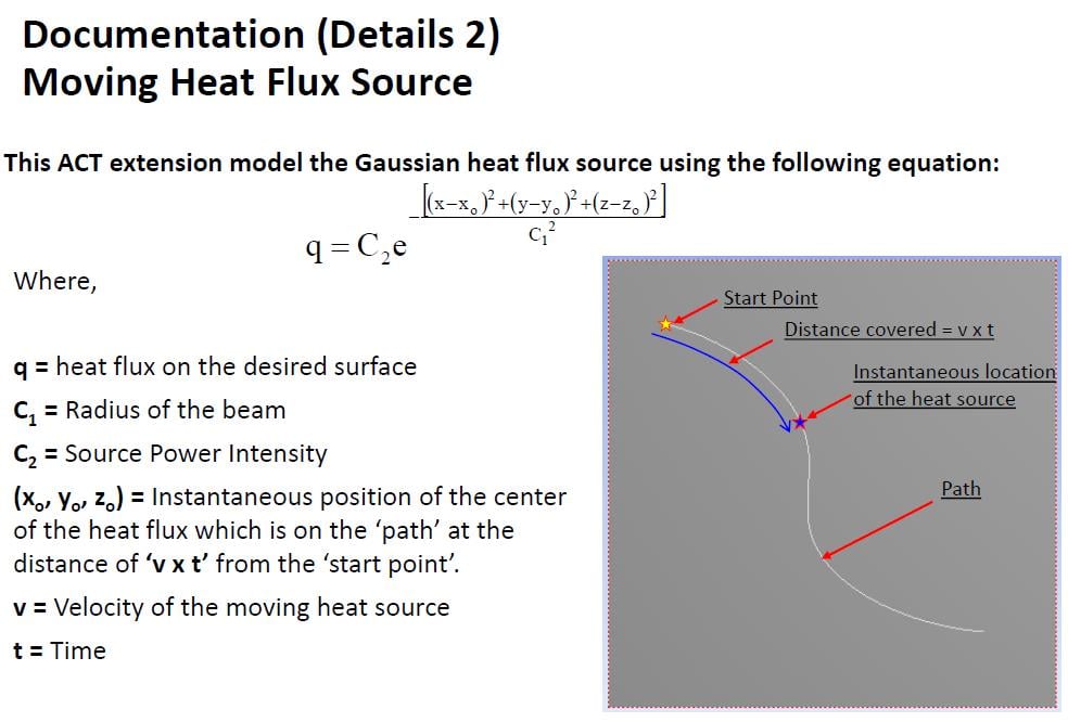
Do you have the documentation? It should be available in the 'doc' folder of the downloaded extension. He is defining heat flux based on the following relation:
Let me know if this helps?
Regards,
Sandeep
-
August 13, 2018 at 1:45 amSubscriberHi Sandeep, yes I have this documentation. Thank you it helps. How should I define C2? Power/laserarea, as I mention above? Also, for a symmetric BC should I use half of the laser area in the flux definition vs. the whole area? Thanks Kellen
-
August 13, 2018 at 3:43 pmAnsys Employee
Yes, I believe C2 is defined by Power/LaserArea.
I don't quite understand your question with respect to symmetric B.C. Is your laser path being affected by the symmetric b.c?
If so, wouldn't the overall path covered by the laser be smaller? Why would the laser intensity have to change for this?
~Sandeep
-
August 13, 2018 at 3:54 pmSubscriber
Sandeep, sorry for any confusion I will try to re-explain. I think my question is more on the concept of the symmetric boundary condition, and how to define a total surface flux if only a certain portion is physically modeled.
My model is simulating half of a single-track deposit width and is symmetric along the center of the laser spot, as it is traversing the surface of the material. Because of this, my model is really only being affected by half of the laser, as the other half is not physically modeled. So when I define the laser intensity as Power/LaserArea, does this mean I need to input Power/(pi*laserradius^2) or Power/(0.5*pi*laserradius^2), i.e. including the entire laser area or only half of the area.
Any information helps.
Thanks
Kellen
-
August 13, 2018 at 4:32 pmAnsys Employee
Kellen, I misquoted earlier here today, please see my edited response below:
[EDITED]:
I would recommend you to make sure that you are capturing half the area? So yes, it would be Power/(0.5*pi*radius^2). When you make it symmetric on the exact edge, you are modeling 2 lasers with a smaller radius, but we still want to capture the total area captured by the whole laser?
I would recommend you to try 2 test cases to confirm if you are getting similar results, One with the full body and one with the symmetric condition defined on the edge? Is this possible?
Regards,
Sandeep
-
August 13, 2018 at 4:35 pmAnsys Employee
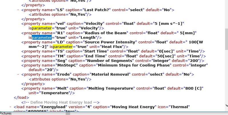
Also,
With regards to parametrizing a variable just open the xml file (in the folder ~CT_MovingHeat_R170_v4.1MovingHeatsrc) and for the input you want to parametrize just add isparameter="true".
Regards,
Sandeep
-
August 13, 2018 at 11:01 pmSubscriber
Hi Sandeep,
Do I need to reinstall ANSYS or do anything additional for the parameterization to work? I input that line of code into the correct folder and am not seeing the parameterization checkbox.
Any info helps, as always.
-
August 13, 2018 at 11:04 pmSubscriber
This is what my xml and input screen show
 up as:
 -
August 13, 2018 at 11:07 pmAnsys Employee
Kellen, can you try uninstalling from the ACT start Page and re-install that extension again?
-
August 13, 2018 at 11:16 pmSubscriber
I did, it did not work. One thing that might not be right is that I have stored the extension in the same folder as my ansys results files. Should the extension (.webex) be saved in the same folder as the ANSYS program is saved?
Kellen
-
August 14, 2018 at 1:42 amSubscriber
Hi Sandeep, another question I have about residual stress analysis is there a simple way to incorporate annealing of Ti6Al4V (i.e. when the annealing temperature is reached, displacement is equal to 0)?
Thanks as always,
Kellen
-
August 14, 2018 at 2:07 amAnsys Employee
Kellen,
I will have to debug a little w.r.t parametrizing the model. I will keep you posted as I find out.
For Annealing, please try EKILL/EALIVE. There are numerous discussions in the forum on this. Try and include a blank load step after EKILL and use EALIVE. Please see this article and this discussion on XANSYS.
P.S: If you have found a solution to your initial query, please mark it as a solution (even if it is your own post) so that it would make things easier for someone going through it at a later time. Also, please post new questions as a new discussion and provide a link to the old discussion.
Regards,
Sandeep
-
August 14, 2018 at 1:24 pmAnsys Employee
Kellen,
Here's what you do to get it to work:
1. Add the isparameter to the variable of interest in the xml file (recommend you to do this in the original download). In this case, I selected Radius and the Source Power Intensity:
2. Next, copy that file MovingHeat.xml and the folder MovingHeat found in the src folder to
%appdata%ansysv191ACTextensions
Replace anything there although I think you would need just the xml file placed there.
3. Once you re-launch Workbench, select the Scripted MovingHeat extension instead of the Binary one.
4. Now once you re-launch Workbench, you will observe the parameter buttons appear:
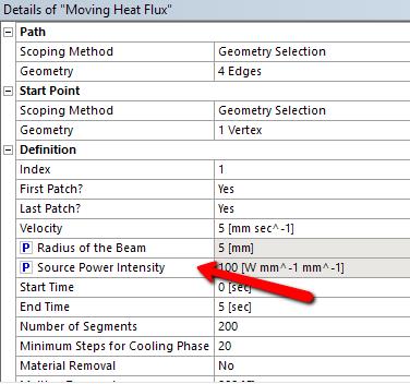
Hope this helps.
Regards,
Sandeep
-
August 14, 2018 at 2:44 pmSubscriber
Hi Sandeep, it worked!
Thanks and I will post on a new discussion when I have further questions.
Regards,
Kellen
-
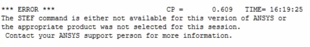
August 14, 2018 at 11:33 pmSubscriber
Hi Sandeep, i wanted to point you to my question posted elsewhere: /forum/forums/topic/stef-error/
-
May 19, 2019 at 6:40 am
Karldekruyf
SubscriberHi Sandeep, I am having a VREAD error when also using MovingHeat. I was wondering if you would be able to assist me with this?
-
May 19, 2019 at 6:43 amSubscriber
I have installed the MovingHeat extension as per the instructions above, and have established my model using the included MovingHeat_help.pdf file. When I attempt to solve my model a VREAD error occurs when the solver is accessing the velocity array. What would be the best way to resolve this?
Thank you,
Karl Dekruyf.
-
April 23, 2020 at 7:53 pm
sunil.voleti
Subscriberhai kellen,
I am simulating laser like you with extension could you please explain me how did you defined Absorption rate or absorption coefficient for simulation.
Thanks in advance.
-
April 23, 2020 at 7:56 pmSubscriber
Hi sandeep could you please expalin me how we can define absorption rate or absorption coefficient when I am using moving heat source(moving heatflux) extension for my simulations.
Thanks in advance
-
April 23, 2020 at 8:21 pmSubscriber
Hi Sunil, simply multiply the overall heat flux (you calculated based on laser parameters and instructions within the toolbox .ppt itself) by the absorption coefficient (found in the literature depending on the material). Then input this value into the ANSYS toolbox instead of the value calculated without taking into account the absorption ratio.
Best,
Kellen
-
April 29, 2020 at 9:45 amSubscriber
Hi Kellen,
Thanks for your answer. could you please explain me in detail about your last answer how we can input absorption rate in moving heatsource extension (moving heatflux) in ansys. and can you please also explain
In transient thermal analysis there is option to select Tabular data for convection which is already defined with in the application with this equationq/A=h(ts -tf) ,I would like to know what is the film coefficient (h) used by ansys for this convection tabular data.Or else could you please explain how did you calculated film coefficient for your simulations.
Thanks and Regards,
sunil.voleti. -
June 5, 2020 at 1:50 pm
tpaplham
SubscriberHi Sandeep,
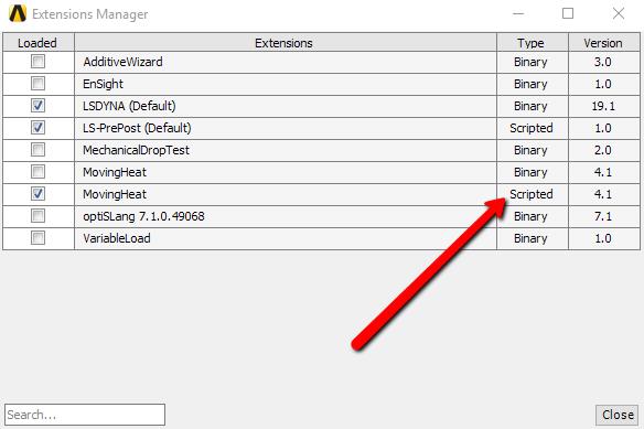
You mentioned that because the Moving Heat Source extension contains source code, it should run in any version of ANSYS even though it is only stated to support ANSYS 17. I am currently trying to run it with ANSYS 19 R2 and get this error when I try to solve:
Is there some other issue that would be causing this?
Thank you,
Tyler
-
December 22, 2020 at 3:26 am
YipKangWei
SubscriberHi Kellen and Sandeep,
I am a student currently working on single layer simulation for AM, I am also using the moving heat source v4.1 extension. I wanted to ask if it is indeed true that the moving heat source utilizes an element birth and death technique? Currently, I am using the element birth and death function in transient thermal separately to account for the "unprinted material" but have been facing errors like "An internal solution magnitude limit was exceeded. Please check your environment for inappropriate load values or insufficient supports." The error usually occur at the element in which I first killed.
Any help or clarification would be greatly appreciated. Thank you!
Regards,
KangWei
-
September 12, 2021 at 2:44 pm
Alp
Subscriber.Hi,
what if one wants to simulate it for 60 second while using the same parameter? For instance, heat source will travel the same path untill the 60 sec is over. Heat source in this case will travel the same path over many times to complete the 60 sec. So what do you think about it? How the parameters should be changed to adapt this situation?
BR,
Alp.
. -
October 17, 2023 at 3:34 pm
Joshua Bakes
SubscriberHello,
I am also using the moving heat source extension in ANSYS (2023 R1) to try and simulate a laser welding process.
I am trying to simulate the laser passing through a highly transparant body (presumably this means a low absorption coefficient) and welding it to another body underneath which has a very low transparancy (high absorption coefficient) so absorbs the lasers energy. My outputted results are temperature, total heat flux, mean temp and material removal.The issue I am encountering is that no matter what values I use for the absorption coefficients in the moving heat energy there is no difference in any of the results, which is leading me to believe that the absorption coefficient doesn't change anything but I am sure this is not the case and there is a problem.
Any help regarding this issue would be massively appreciated.
Many thanks
Josh
-
- The topic ‘AM Single Layer Simulation’ is closed to new replies.


-
peteroznewman
 5874
5874 -
scabo
 1906
1906 -
Dennis Chen
 1420
1420 -
javat33489
 1306
1306 -
Shyam Prasad V Atri
1021


© 2026 Copyright ANSYS, Inc. All rights reserved.
