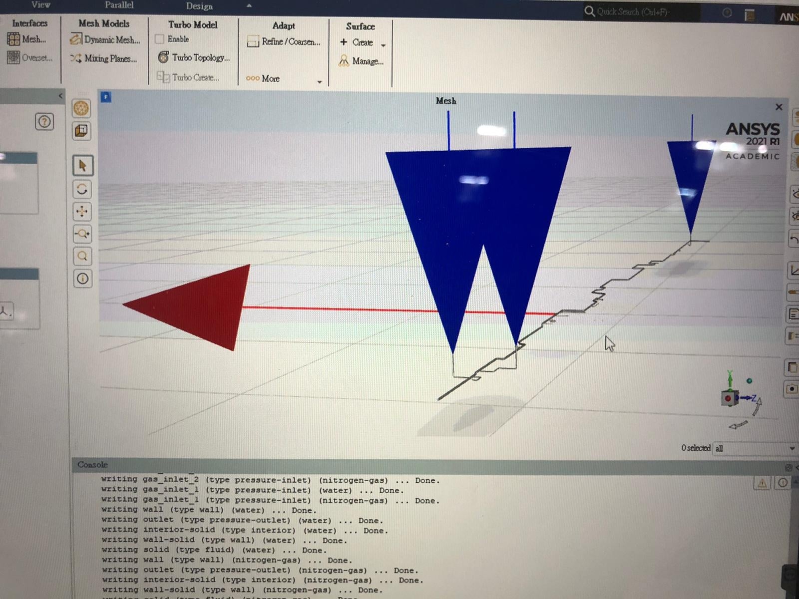
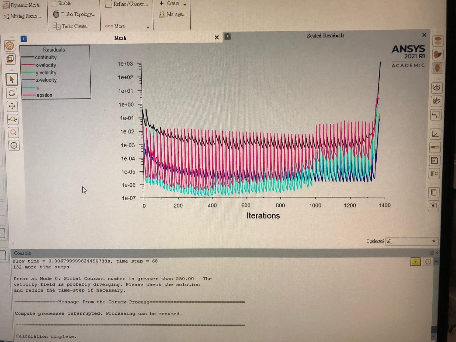
-
-
June 29, 2021 at 7:51 am
Jason Sum
SubscriberJune 29, 2021 at 1:32 pmKarthik Remella
AdministratorHello To be honest with you, the choice depends on the nature of the problem as well as how strongly (or weakly coupled) your governing equations are. If you have a stiff set of equations, you are better off using a Coupled solver. Otherwise, any segregated solver might work. If you are solving a transient problem, I would go with PISO (if I believe right). To read more about this, I'd recommend that you refer to the following link from Ansys Help.
https://ansyshelp.ansys.com/account/secured?returnurl=/Views/Secured/corp/v211/en/flu_th/flu_th_sec_uns_solve_pv.html
Karthik
June 29, 2021 at 3:02 pmRob
Forum ModeratorI'd be more concerned about the mesh resolution if you're using the mesh from here /forum/discussion/29218/why-i-was-banned-to-proceed-to-setup-after-meshing-even-i-fulfilled-the-student-ver-limit-of-512k#latest it's very likely too coarse to get a decent solution. Work out your cell courant number and plug flow residence time too: this might be a very long run.
June 30, 2021 at 2:04 amJason Sum
SubscriberMy geometry is large in size which makes meshing coarse while fulfilling the upper limit of 512k elements.
Would you mind explaining further on how to get a better result by looking into cell courant number and flow residence time, thanks so much Rob and Karthik!
I found that when COUPLED is chosen as the solution method, under 'Control', the flow courant number is 200 now, which I know the desired value should be less then 1. What should I do to reduce the flow courant number (or just directly change it to my desired value) and what to do with the flow residence time on Fluent?
June 30, 2021 at 10:45 amRob
Forum ModeratorThe default is 200, which is fine for external aero flow, and far too aggressive for anything interesting, 20-50 is more reasonable for multiphase.
The values I suggested you look at will help estimate the time step you need, then the number of time steps. It's partly to assist in choosing the settings but also allows an estimate on the total run time. With that you can decide if it's feasible in the time you have.
If you want to use multiphase you need to resolve the phase gradient. Otherwise the results may be misleading. If the system is fairly level can you use a residence time approach? Look for "mean age of air" on here as it's a method that's been abused for years in many applications.
July 5, 2021 at 8:16 amJason Sum
SubscriberSorry that I do not have much understanding on phase gradient, I am kind of newbie to Ansys Fluent! Really need your guidance ! Thanks Rob!
As my elements and nodes cannot be smaller due to the limit of student version, as you said, what I can do is working on the courant number. Am I supposed to try inputting different Time Step Size and see the global courant number shown from the console, until a trial the courant number obtained is within 20-50 as you suggested? So that I can confirm my proper Time Step Size and determine the Number of Time Steps based on how long I want it to simulate in actual world?
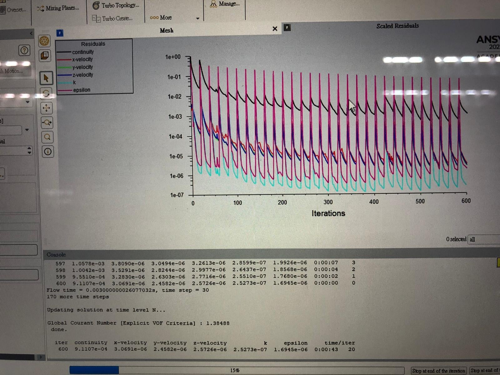
The following residual graph shown having set up of Number of Time Step = 200, Time Step = 0.0001, Max Iteration = 20, obtaining courant number between 1 - 2 values .
(Solution method: PISO with default setting, Control: default setting)
(Three Nitrogen gas inlet with Gauge Total Pressure of 34474Pa and Supersonic/Initial Gauge Pressure = 34400Pa)
What is this graph implying? The k and epsilon curve keep fluctuating, is this meaning a undesirable result? What should I do to obtain convergence, thanks!!!
July 5, 2021 at 10:14 amRob
Forum ModeratorWith PISO you want to get the VOF courant number to be around 1. The default courant number of 200 is part of the pressure based coupled solver, and is a setting you add: which was in answer to the question above my earlier post. You have since switched to PISO which is generally better for transient applications.
The above residual plot is because you're using the transient solver. We solve for each time step, and the spike is when we increment time and move onto the next step before we then converge each step.
July 5, 2021 at 12:08 pmJason Sum
SubscriberOhh! So are the residual graph attached above and my setup for this simulation (pumping N2 to pump water inside away) on the right track? Or any symptoms from the curve can be seen that my setup is inaccurate? Thanks Rob again!
July 5, 2021 at 4:16 pmRob
Forum ModeratorYou've run 0.003s so it may be a bit early to draw any conclusions from the results!
July 6, 2021 at 12:57 amJason Sum
SubscriberJuly 6, 2021 at 4:58 amJason Sum
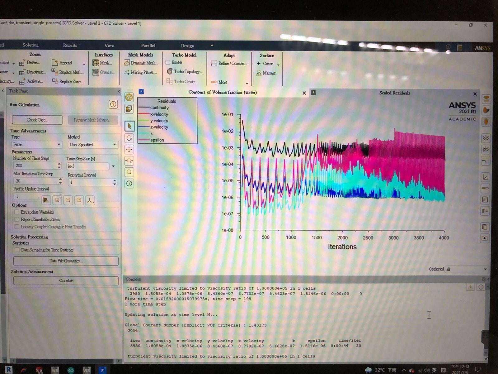
SubscriberI reduced the time step size from 1e-4 to 8e-5 and ran the calculation again, the attached is the residual graph!
Initially the residuals tended to drop and converge, but after around 1000th iteration, the graph became like this. What can I do to modify so that convergence can be obtained? Thanks for your help!!!
July 8, 2021 at 6:28 amJason Sum
SubscriberIt is sincerely hoped for solutions and guidance from forum experts! Many thankss.
July 8, 2021 at 10:42 amRob
Forum ModeratorHave a look at the flow field and see if there are any regions with "odd" velocity vectors or poorly resolved gradients. They're usually an indicator of where things are going wrong.
July 9, 2021 at 3:17 amJason Sum
SubscriberShould I set an animation for the velocity vectors, searching for the "odd" parts from it after calculation? Is Adaptive Time Stepping more preferable in my case (multiphase) for calculation? Thanks a lot!
July 9, 2021 at 1:08 pmRob
Forum ModeratorAnimations can help diagnose problems, but just having a look at the flow is often enough.
I generally avoid adaptive time stepping. It's an excellent idea in principle but as it relies on the solver spotting it's diverging before it fully diverges. Depending on the flow field that may not happen!
July 11, 2021 at 2:06 pmJason Sum
SubscriberI am struggled on where to observe the flow field and how to figure out the "odd" parts? Am I supposed to observe the contour about velocity to see any odd parts? thanks!
July 12, 2021 at 10:59 amDrAmine
Ansys EmployeeCreate cell registers using Field Variable and provide ranges for velocity etc to identify places where you have overshoots. Moreover: just look into 5 to 10 time steps (under Residual Monitor reduce the number of iteration to be plot) otherwise you won't figure out if you are converging in each time step or now.
Also enable the physics constraint for adaptive time stepping.
July 14, 2021 at 7:36 amJason Sum
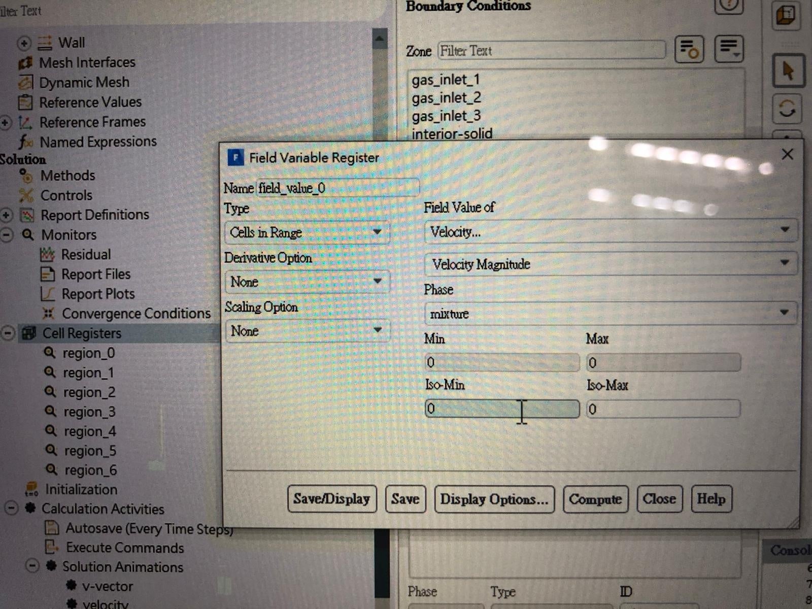
SubscriberThanks Amine. As shown above, the epsilon curve in residual graph keep spike higher and higher. How can I identify the problematic region(s) (causing the residual not converging) after setting cell registers?
In the following photo, what range should I set for the velocity magnitude so that I can find out the error of my setup? Thanks a lot!
July 14, 2021 at 12:53 pmRob
Forum ModeratorThe range you choose is model dependent. Look for regions that are fast compared to the expected velocities.
July 14, 2021 at 3:51 pmDrAmine
Ansys EmployeeCase dependent and you need to feel reasonable value range which either by boundaries or by physics or even both.
July 19, 2021 at 8:10 amJason Sum
SubscriberAfter running calculation with 200 time steps with time step size = 4e-5 and max iterations/ time step = 40, below is the residual graph obtained:
 (Figure 1. Residual graph)
As guided, I set a field variable in "Cell Register" with velocity magnitude, found that the range of velocity for the whole model = 0 - 175, while only the following part especially having velocity range of 100 - 175.
I also set Turbulent kinetic energy k in "Cell Register" as field variable and found that the following part having especially highest k value.
Does it mean that I should mesh this part with finer nodes, or any further actions I can do to obtain a converging k value in residual graph and an accurate solution? Thanks a lot!
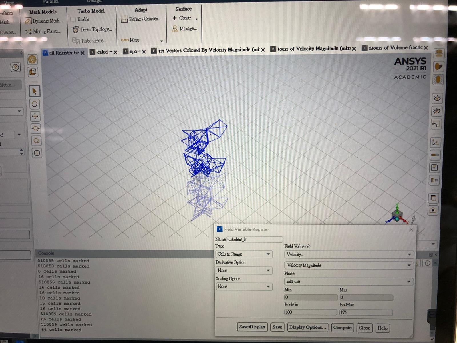 (Figure 2. Specific part found to have "odd" velocity)
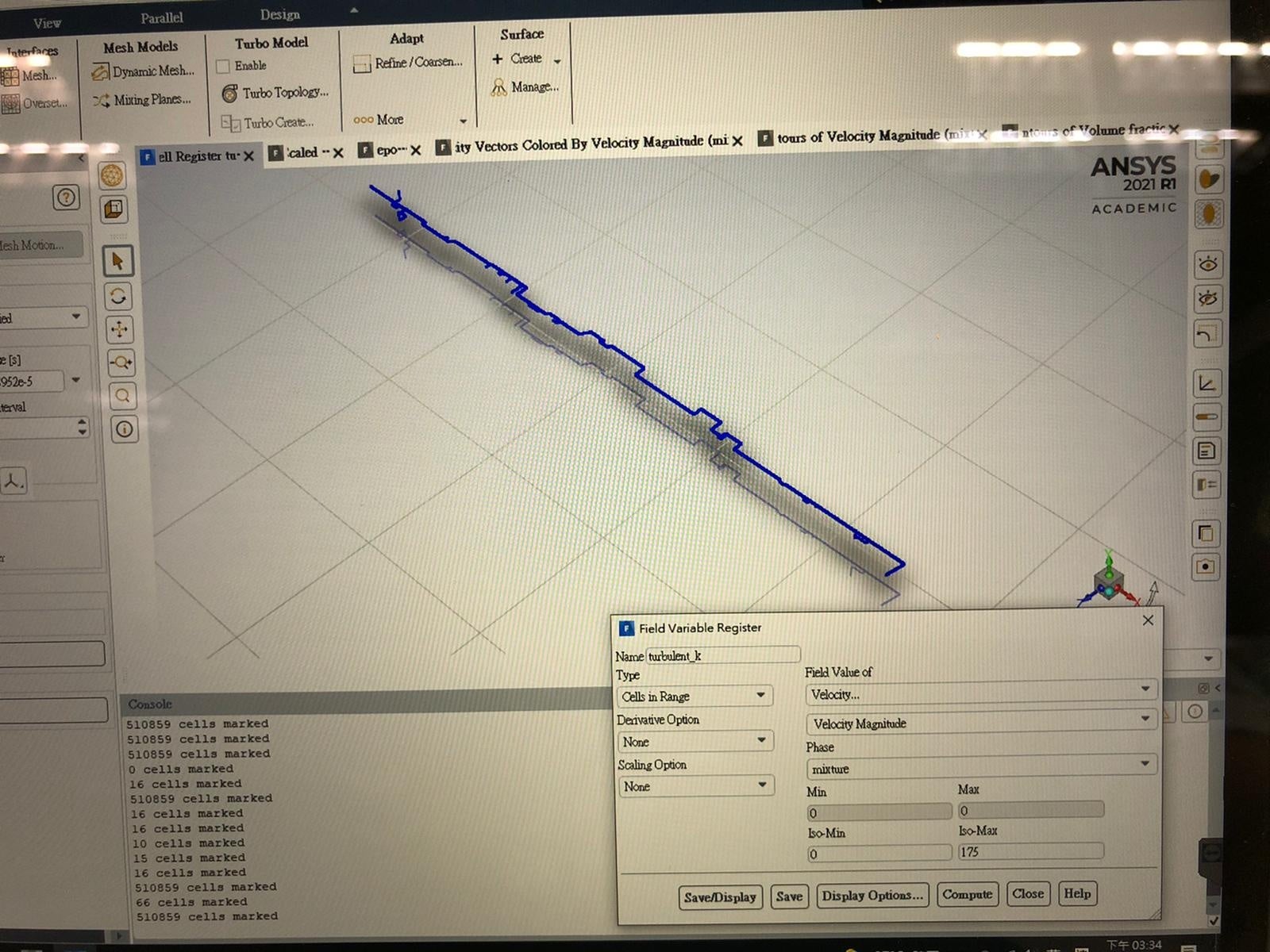 (Figure 3. The velocity magnitude range of whole model)
July 19, 2021 at 8:20 amDrAmine
Ansys EmployeeAre you expecting this high velocity?
July 19, 2021 at 4:09 pmJason Sum
SubscriberI am not sure the velocity of particular point throughout the model. just knowing that each inlet pressure is 5 psi.
I deduce the above part (Figure 2 above) is the "odd" part of my model because the cells with top 70% of velocity magnitude of the model are from this part, which seems abnormal.
Also as the k value in residual graph spike up with greater fluctuation along the iteration, I found that the suspected "odd" part (Figure 2 above) having especially higher k value from cell register.
Should I improve the meshing quality of that part and try observe the residual graph again? I am not sure am I going on the right path, thanks for your help further!!
July 20, 2021 at 7:46 amDrAmine
Ansys EmployeeThat is a good path.
If using VOF you can set a velocity limiting to avoid this kind of "abnormal" velocities.
July 20, 2021 at 9:10 amJason Sum
SubscriberNow that I targeted that "odd" part, should I step back to the meshing and mesh that part with finer elements, OR setting a velocity limiting as you proposed? How to do so? Thanks!
July 20, 2021 at 10:38 amRob
Forum ModeratorYou really need a finer mesh everywhere. Refining that region will help for now but I suspect the problem will move elsewhere.
July 21, 2021 at 7:13 amJason Sum
SubscriberThanks Rob! I will try to refine the whole model first! By the way, I would like to ask for such huge model (a underground gas pipe network with ~100m long, 12'' diameter), how or any indicators to determine a proper element size of the whole model and how fine should I adjust?
Should I keep inflation meshing layer of 5, and refine the body sizing?
Will it be better if elbows are having especially finer meshing?
July 21, 2021 at 7:18 amDrAmine
Ansys Employeeanyway where you expect rapid changes and steep gradients keep the resolution fine enough to avoid huge jumps!
July 21, 2021 at 10:00 amJason Sum
SubscriberOkay! Thanks Amine! To obtain a desirable meshing quality, should I keep trial and error to review the residual convergence from calculation on Fluent? If convergence doesn't reach in residual graph, am I supposed to return to Meshing step to refine the model? Once convergence reached, meaning the meshing size and density are enough?
July 21, 2021 at 10:50 amRob
Forum ModeratorSort of. You have to resolve the flow (and gradients) spatially (mesh) and temporally (time step) so it's a bit more complicated. Adding in secondary phase(s) makes it even more fun. You have a relatively small system, so we'd model with a lot of mesh: if you extend to kilometres of pipeline we'd switch to a network model. Twinbuilder or Modelica are the Ansys tools, but industrially (oil & gas) OLGA is used for that type of simulation. We may then couple into OLGA for complex components.
July 22, 2021 at 1:47 amJuly 22, 2021 at 8:51 amRob
Forum ModeratorHave a look to understand why they're skew: I'd not expect the mesher to struggle with the CFD settings in a pipe!
July 26, 2021 at 4:01 pmJason Sum
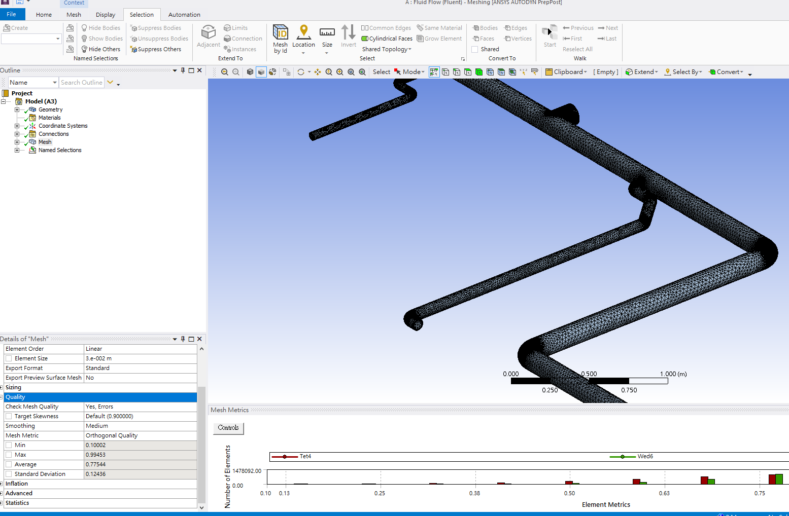
SubscriberBy using standard version, I have already meshed the whole pipe network with way finer body sizing meshing with 5 layers default inflation, while the elbows and tees were refined with more fined surface sizing meshing.
Body meshing element size : 3e-2
Elbows and tees element size: 5e-3
Node: 2635812
Element: 7373330
Quality Mesh Metric:
Orthogonal Quality: mainly ranging 0.75 - 0.9
Skewness: mainly ranging 0 - 0.25
Hybrid Initiation with water patched inside the pipe model
Method: PISO
Control: Default Under-relaxation factor
Boundary Conditions: 3 Inlets with each 5 psi Nitrogen gas pumping into the pipe network to simulate pumping water out of the only outlet
Time Step: 200
Time Step Size : 4e-5
Max iteration/time step : 40
1st iteration :Global Courant Number [Explicit VOF Criteria] : 5.1802
1189th iteration : Global Courant Number [Explicit VOF Criteria] : 2.24168
Below is my residual graph of calculation from 1st to 1189th iteration. Here are two questions hope for answer! Thanks!!!
I would like to ask, after refining, is the residual graph below satisfactory and is it reaching convergence?
When every time step complete, I saw it showed "solution is converged", does this indication mean my setup already having reliable simulation and obtaining residual convergence
July 26, 2021 at 4:29 pmRob
Forum ModeratorPlease post a couple of screen shots from the movie - I'm not permitted to open it.
If every time step is converging then there's a good chance the solution is reliable. However, you also need monitors of mass etc to confirm.
July 26, 2021 at 4:34 pmJuly 26, 2021 at 4:37 pmRob
Forum ModeratorLooks reasonable. How are the balances, and how sensible do the results look? Note, inflation tends to result in a fairly high aspect ratio which then causes problems, you may find you need to resolve near the wall and in the streamwise directions at much the same resolution.
July 26, 2021 at 4:46 pmJason Sum
SubscriberOkay! I will try resolve the inflation parts.
By the way, how can I check the balance?
Also, now actual physical flow time merely = 200 x 4e-5 = 0.08s, which actually need wait for the computer to run for about 36 hours
In my case, what do you suggest so that the calculation can be way faster? (Like reduce meshing density or any other possible solution?) I am only having 6 core and GeForce GTX1650 4GB equipped. Thanks!!
July 27, 2021 at 9:25 amRob
Forum Moderator36 hours isn't too bad, other than more parallel & faster cpu there's not much you can do. Using a coarser mesh will speed things up, but you'll just produce rubbish faster. Some models run in a few 10's of minutes, others can take several weeks or even months: CFD isn't always a quick process.
Re the balance, you need to look at the mass fluxes and volume integral: what goes in must come out or add to the volume mass.
July 27, 2021 at 1:17 pmJason Sum
SubscriberTwo questions would like to seek for your further help:
I have set 4 parallel solver in the box before launching fluent, which made my fluent calculation faster! Now 0.08 s real world simulation only took around 12 hours! I would like to ask what parallel means, does my 6 core cpu mean that I can set max. 6 parallel solver?
Below is my calculation using 4 parallel solver:
Time step size: 3e-5
Time step: 200
Max. Iter/time step: 40
1st Iter: Global Courant Number [Explicit VOF Criteria] : 5.18633
last Iter: Global Courant Number [Explicit VOF Criteria] : 1.42208
 2. I have also plot a mass imbalance graph during calculation, based on the below graph and above transient residual graph, do you think the setting is now reliable with residual convergence and I should keep this setting? Many thanks Rob!!!!!!

July 27, 2021 at 2:27 pmRob
Forum ModeratorThat looks promising, but you'll need to check velocity etc and that the results make sense. It's hard to give a definite answer without reviewing the case and we're not able to do that.
Re the cores. The solver has 4 cores parallel as part of the Student licence. So that's the limit. Research and commercial licences also allow access to (additional) HPC packs so you can run many cores depending on the number of packs that are bought.
July 27, 2021 at 2:41 pmJason Sum
Subscribersame way as monitoring above mass imbalance to monitor by plotting graph of the velocity magnitude?
in case without educational license limit, say a 6 core cpu at most can have how many parallel solver? Six? Thanks!!!
July 27, 2021 at 4:04 pmRob
Forum ModeratorOn your machine, with a suitable licence, 6 would be the maximum. Depending on the cpu and boards you should see good (near enough linear) speed up. To give you an idea KAUST ran on 200k cores a couple of years back: we run 2-300 cores regularly here.
July 28, 2021 at 6:36 amJason Sum
SubscriberNow that the residual convergence and mass imbalance were deduced to be reasonable, for checking the velocity or other variable, should I plot to monitor them just like monitoring mass imbalance, OR just observe their range in cell register? Thanks!
July 28, 2021 at 10:36 amRob
Forum ModeratorJust monitor. In CFD we monitor residuals, monitors and fluxes. Once the computer says the model is done we also manually check the result: that is to check that the result is "correct" as the other checks are that the solver has done it's job, not that the boundary conditions etc are sensible.
August 2, 2021 at 9:36 amAugust 2, 2021 at 2:55 pmRob
Forum ModeratorYes! I tend to monitor velocity/temperature/phase on a point to see how much it's changing. Your case is more complex as you may have several phenomena interacting at different frequencies.
August 3, 2021 at 7:26 amAugust 3, 2021 at 7:29 amDrAmine
Ansys EmployeeCheck the underlying objects behind that velocity animation sequence.
August 3, 2021 at 7:37 amJason Sum
SubscriberI already selected all inlets, outlet and wall of the model for the velocity magnitude,. Suppose the pipe contains some water inside, if inlets having pressure pumped inside, there should be water movement and velocity gradient changes showing, but throughout the animation stored, the wall of model keeps in blue colour. Thanks for help!!!

August 3, 2021 at 10:52 amRob
Forum ModeratorWhat should the fluid velocity be at the wall? Think carefully! Try the same plot with node values off.
August 3, 2021 at 11:32 amDrAmine
Ansys EmployeeIf you select velocity contour at just inlet what do you see? Velocity is zero at walls if they do not have motion. What are your Inlet boundary conditions?
August 7, 2021 at 5:41 amJason Sum
SubscriberThanks both of you!
In the velocity contour, I saw the inlets (cross section of pipe) having velocity color gradient changes!
My boundary condition:
Three risers inlets each having 5 psi total pressure with nitrogen pump in.
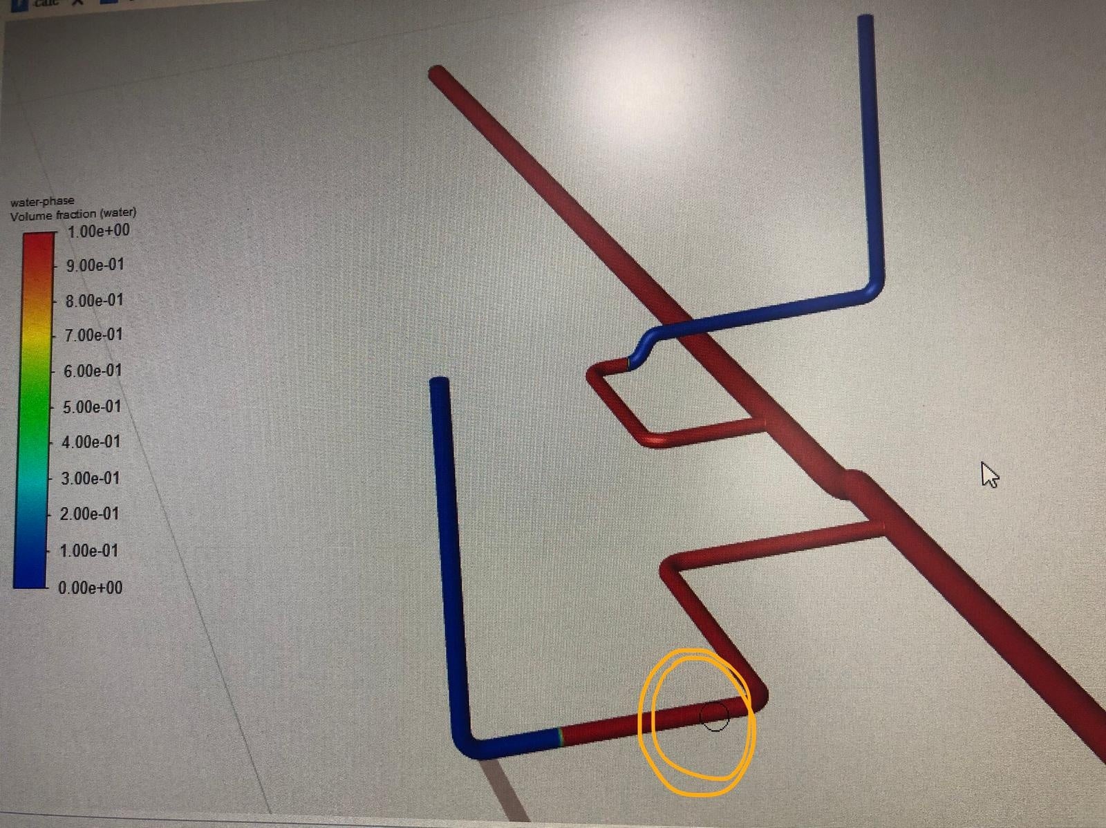
I ran the calculation again by plotting a graph of Area weighted average velocity magnitude of mixture at the point circled below.
I would like to ask after obtaining the graph of velocity at a point, how can I determine it makes sense and it is a reliable result?
 The point:
August 9, 2021 at 10:56 amRob
Forum ModeratorCompare the monitor with expected values. If the result is converged the value will be numerically correct, but you'll need to apply good engineering to confirm the results are physically sensible for your intended settings.
It's the old question. We test the solver, so we're confident the result is correct. What we can't say is if you put all the boundary conditions & material properties in correctly.
August 15, 2021 at 2:17 amJason Sum
SubscriberOkay Rob! I will confirm the result by apply own engineering calculations and sense.
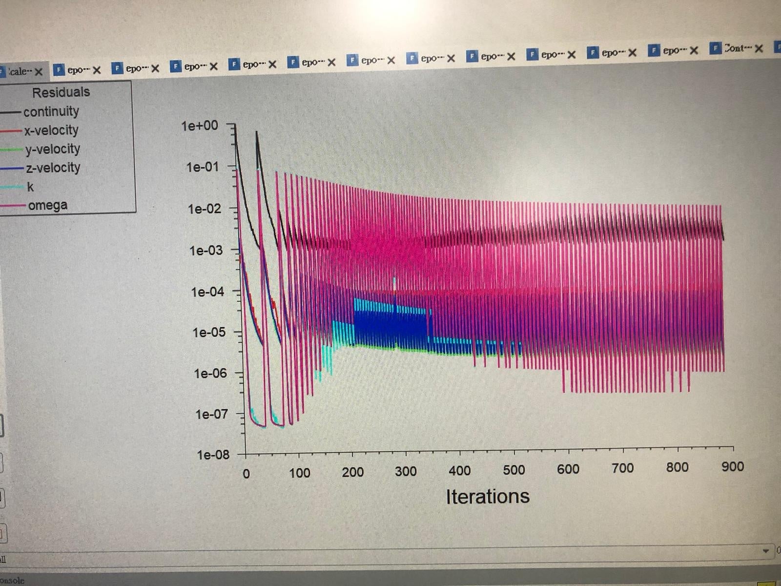
I ran a calculation with time step size of 3e-5 with 400 time steps, and max iter of 40.
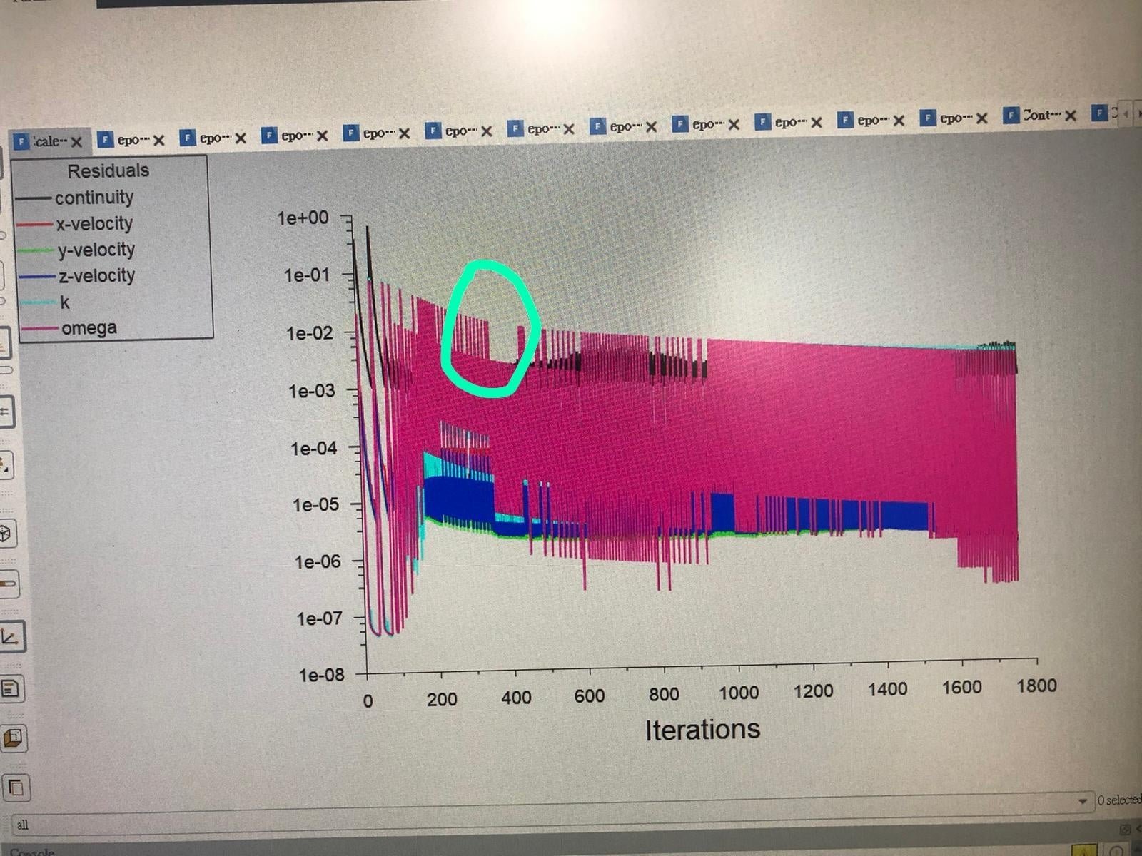
The first graph below shows the 900 iteration is seemingly converging for transient, but when it keep calculation further with increasing iterations, for 2nd graph, the 0-900 iterations already not same as the 1st graph. 0-2000 iterations in 3rd graph even seems like being skewed. What's wrong with it and why? Thanks!!!

August 16, 2021 at 12:18 pmJason Sum
SubscriberSincerely seeking for answer with many thanks!
August 16, 2021 at 12:51 pmRob
Forum ModeratorYesterday was Sunday: I only work for my wife on Sundays.....
It's data retention, Fluent stores the last 1000 (by default) residual points so anything beyond that may look a bit odd. Nothing to worry about.
August 16, 2021 at 12:55 pmJason Sum
SubscriberOhh!! Sorry Rob! I mess up with the time difference!
thanks for your professional answer! You helped a lot! Have a good day!
August 16, 2021 at 1:00 pmRob
Forum Moderator:) Thanks, you too.
Viewing 57 reply threads- The topic ‘Which solution method (scheme) should I select for multiphase flow (pumping gas to blow water out)?’ is closed to new replies.
Innovation SpaceTrending discussionsTop Contributors-
5664
-
1890
-
1419
-
1304
-
1021
Top Rated Tags© 2026 Copyright ANSYS, Inc. All rights reserved.
Ansys does not support the usage of unauthorized Ansys software. Please visit www.ansys.com to obtain an official distribution.
-
The Ansys Learning Forum is a public forum. You are prohibited from providing (i) information that is confidential to You, your employer, or any third party, (ii) Personal Data or individually identifiable health information, (iii) any information that is U.S. Government Classified, Controlled Unclassified Information, International Traffic in Arms Regulators (ITAR) or Export Administration Regulators (EAR) controlled or otherwise have been determined by the United States Government or by a foreign government to require protection against unauthorized disclosure for reasons of national security, or (iv) topics or information restricted by the People's Republic of China data protection and privacy laws.

