Numerical Results in Fluent
y+
Turbulent flows are significantly affected by the presence of walls. The k-epsilon turbulence model is primarily valid away from walls and special treatment is required to make it valid near walls. The near-wall model is sensitive to the grid resolution, which is assessed in the wall unit y+ (defined in section 10.9.1 of the Fluent user manual). We'll gloss over the details for now and use the following rule of thumb: select the near-wall resolution such that y+ > 30 or < 5 for the wall-adjacent cell. Look at section 10.9, Grid Considerations for Turbulent Flow Simulations, for details.
First, we need to set the reference values needed to calculate y+.
Problem Setup > Reference Values
Select inlet under Compute From to tell Fluent to use values at the pipe inlet for the reference values. Check that the reference value for density is 1 kg/m3, velocity is 1 m/s, and coefficient of viscosity is 2e-5 kg/m-s as given in the Problem Specification. These reference values will be used to non-dimensionalize the distance of the cell center from the wall to obtain the corresponding y+ values.
Let's plot y+ values for wall-adjacent cells to check how they compare with the recommendation mentioned above.
Results > Plots > XY Plot > Set Up...
Make sure that Position on X Axis is set under Options. Also, make sure that 1 is the value next to X, and 0 is the value next to Y and Z under Plot Direction. Recall that this tells Fluent to plot the x-coordinate value on the abscissa of the graph. Pick Turbulence...under Y Axis Function and select Wall Yplus from the drop-down list under that. Since we want the y+ value for cells adjacent to the wall of the pipe, choose wall under Surfaces.
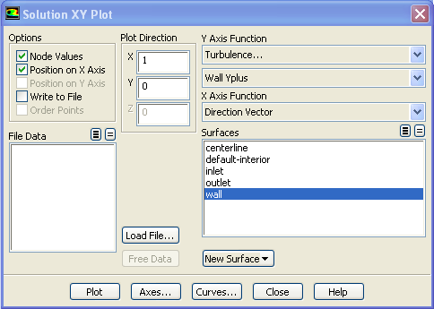
Click Plot.
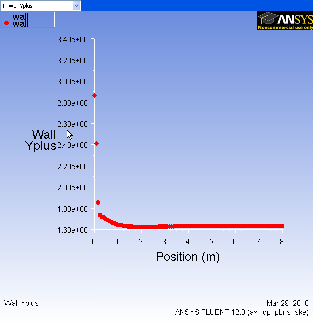
As we can see, the wall _y+_value is between 1.6 and 1.9 (ignoring the anomalous value at the inlet). Since this is less than 5, the near-wall grid resolution is acceptable.
Save Plot
In the Solution XY Plot Window, check the Write to File box under Options. The Plot button should have changed to the Write... button. Click on Write.... Enter yplus.xy as the file name and click OK. Check that this file has been created in your Fluent working directory.
Centerline Velocity
Under Y Axis Function, pick Velocity... and then in the box under that, pick Axial Velocity. Finally, select centerline under Surfaces since we are plotting the axial velocity along the centerline. De-select wall under Surfaces.
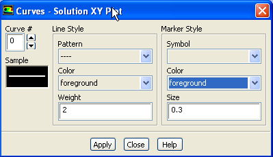
Click on Curves... in the Solution XY Plot window. Select the solid line option under Pattern as shown below. Change Weight to 2. Select the blank option under Symbol. Click Apply and Close.
Turn on grid lines: In the Solution XY Plot window, click on Axes.... Turn on the grid by checking the boxes Major Rules and Minor Rules under Options. Leave Auto Range checked. Click Apply. Select Y under Axis and repeat. Click Apply and Close.
Uncheck Write to File. Click Plot.
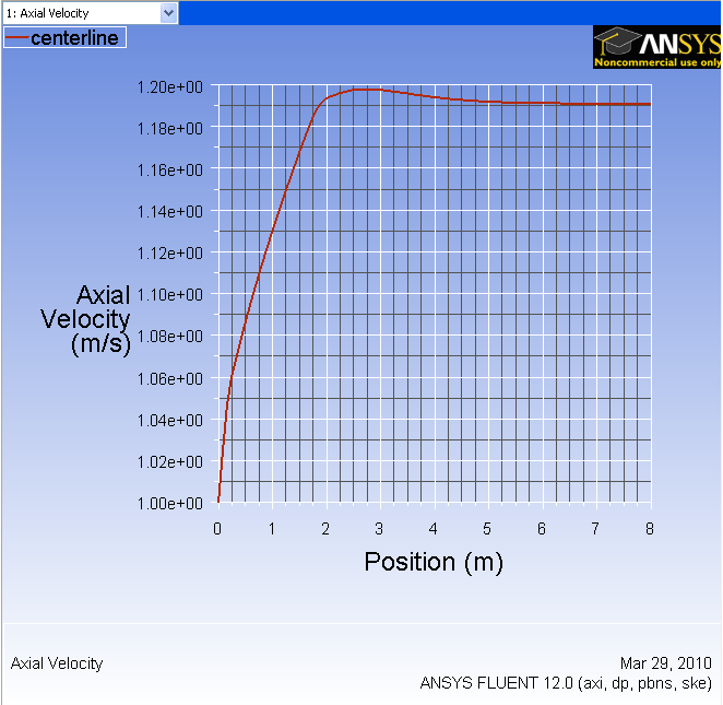
We can see that the fully developed region starts around x=5m with the centerline velocity becoming constant at a value of 1.195 m/s. This is quite a bit lower than the value of 2 m/s for the laminar case. Can you explain the difference based on the physical characteristics of laminar and turbulent flows?
Save the data for this plot as vel.xy.
Coefficient of Skin Friction
The required reference values of density and velocity have already been set when plotting y+.
Go back to the Solution XY Plot Window. Under the Y Axis Function, pick Wall Fluxes... and then Skin Friction Coefficient in the box under that. Under Surfaces, we are plotting the friction coefficient along the wall. Uncheck centerline surface.
Uncheck Write to File. Click Plot.
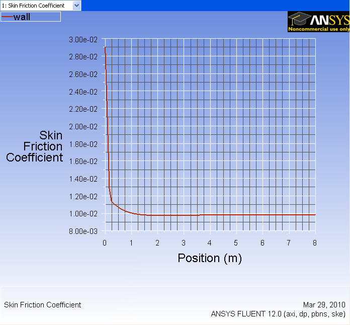
We can see that the fully developed value is 0.0085. Compare this with what you'd expect from the Moody chart.
Save the data for this plot as cf.xy.
Velocity Profile
We'll plot the axial velocity at the outlet as a function of the distance from the center of the pipe.
Change the plot settings so that the radial distance from the axis is plotted as the ordinate: In the Solution XY Plot window, uncheck Position on X Axis under Options and choose Position on Y Axis instead. Under Plot Direction, change X to 0 and Y to 1. For the X Axis Function, i.e., the abscissa, pick Velocity... and Axial Velocity under that.
Since we want to plot this at the outlet boundary, pick only outlet under Surfaces.
Uncheck Write to File. Click Plot.
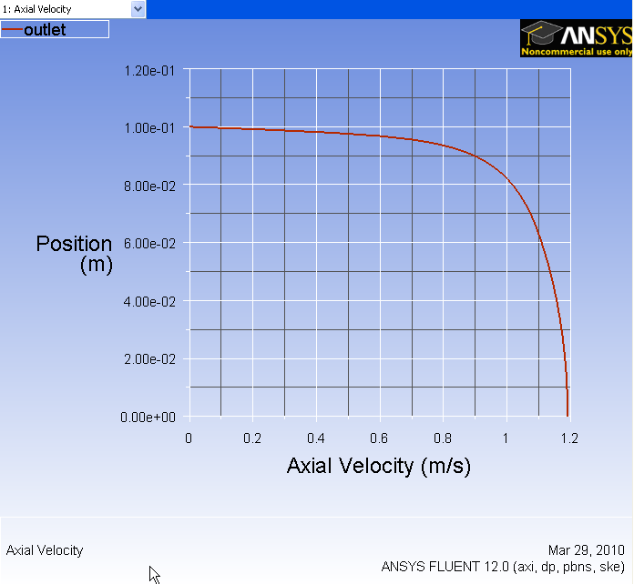
The axial velocity is maximum at the centerline and zero at the wall to satisfy the no-slip boundary condition for viscous flow.
Save this plot as profile.xy.
