Validation & Verification — Lesson 8
To verify the LES solution to the turbulent pipe flow problem, we will compare it against the solution obtained using standard k-e model.
Turbulent Pipe with k-e model
In the Workbench Project Page, left-click on the downward pointing arrow on the top-left corner of the TurbulentPipeLES project and select Duplicate from the drop-down menu as shown in the figure below.
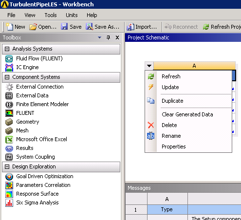
A new project will be created. Rename this new project as TurbulentPipeRANS as shown in figure below.
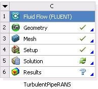
Next, double click on the Solution cell of the TurbulentPipeRANS project. This will launch the Fluent solver. Here we will change the viscosity model to k-e model. In the Fluent window, click on General tab on the left-hand side pane. Choose Steady for Time. Click OK for the pop-up warning. 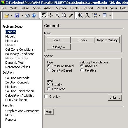 Next click on Models>Viscous on the left-hand side pane as shown below. Choose Edit....
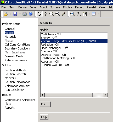
In the Viscous Model window, choose k-epsilon (2 eqn) for Model. Choose Realizable for k-epsilon Model. Choose Enhanced Wall Treatment for Near-Wall Treatment. Click OK as shown in the figure below.

Click on the Boundary Conditions tab on the left-hand side pane. Choose Outlet and click Edit....Change the Turbulence Specification Method to Intensity and Hydraulic Diameter. Set Backflow Turbulent Intensity to 10% and Backflow Hydraulic Diameter to 0.0127 m. Click OK.
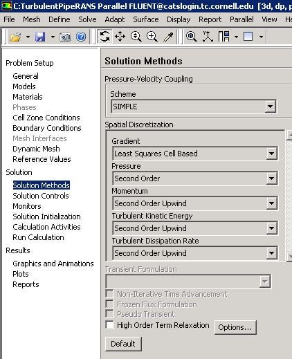
Next, click on Solution Methods tab on the left-hand side pane. Choose Second Order Upwind for Turbulent Kinetic Energy and Turbulent Dissipation Rate.
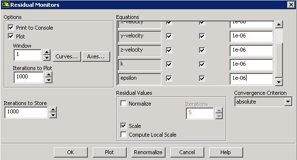
Click on Monitors > Residual and click Edit.... Set 1e-06 for k and epsilon. To get faster convergence, choose 1e-05 for continuity and click OK.
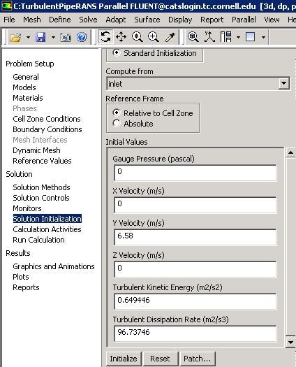
Click on Solution Initialization and click Compute from and choose inlet. Click initialize as shown below
Click on Run Calculation and set Number of Iterations to 1000. Click Calculate as shown below.
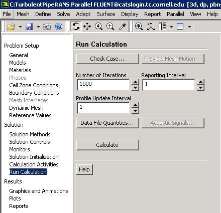
The solution converges in about 600 iterations.
Create Line
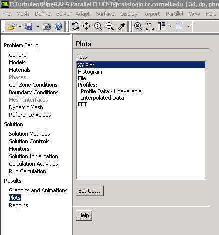
Click on Plots > XY Plot > Set Up... as shown below.
In the Solution XY Plot, choose New Surface > Line/Rake... as shown below.

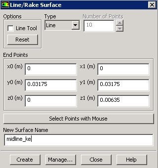
Choose the coordinates of the two points that define the line as below and name the line as midline_ke and click Create and Close the window.
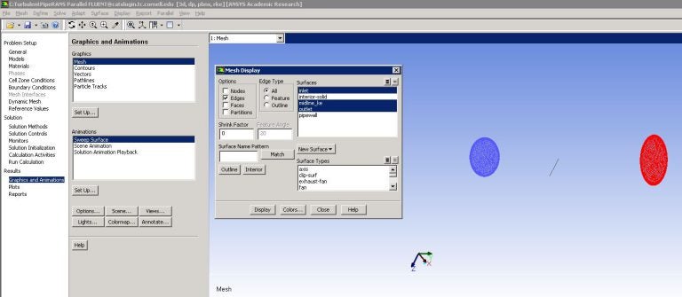
 The line can be viewed by clicking Graphics and Animations > Mesh > Set Up....
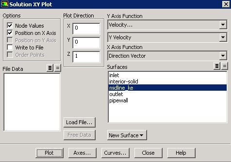
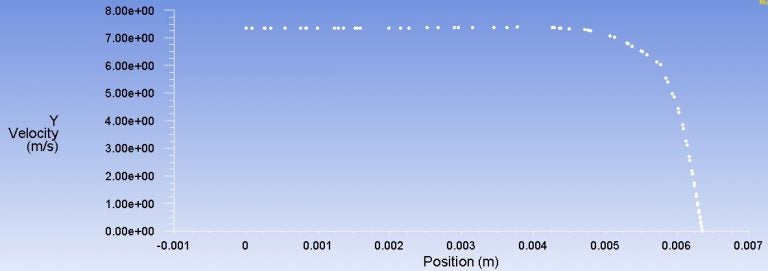
Go back to the Solution XY Plot window by clicking Plots > XY Plot > Set Up.... In this window, choose Velocity... and Y Velocity for Y-Axis Function. Also, choose 0, 0, 1 as the Plot Direction. Finally, choose midline_ke under Surfaces. and click Plot.
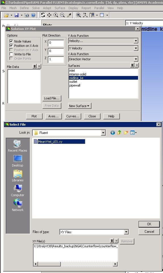
To compare the solution from LES simulation with that from the k-e model, click Load File... in the Solution XY Plot and choose the saved file MeanYVel_LES.xy from the previous section as shown in the figure below.
In the Solution XY Plot select Mean Y Velocity under File Data and click Plot. The figure below shows the comparison of the mean Y velocity from k-e and LES simulations. Both results are very close, which validates the solution procedure for the LES simulation.


