Verification — Lesson 6
The first thing we check for verification is the comparison with the analytical solution since we have one. Then, we do a mesh refinement and use a smaller time-step to check whether the results are consistent with the original calculation. By using a finer mesh and a smaller time-step, we investigate the effects of truncation error caused by spatial discretization and temporal discretization. Then we will do a case comparison for the results obtained after spatial and temporal refinement.
Analytical Solution
Import this csv file and compare it to the Fluent solution at t* = 0.010. You can see how to import a csv file into CFD-Post at 2:46 in the Numerical Results video from the 3D Steady Diffusion tutorial.
Mesh Refinement & Smaller Time-step
It is always a good habit to check that the mesh is refined enough. For example, you could use an element size that is half of what was used in the videos and compare the results.
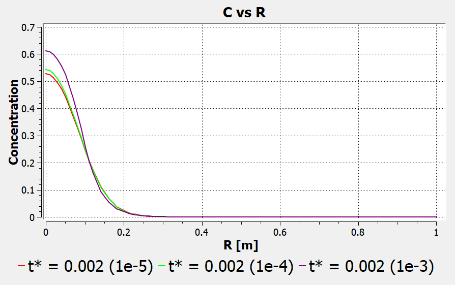
For transient problems, often the time-step size is crucially important in obtaining an accurate solution. For example, in the image below, three different time-step sizes were used and three different results were obtained:

However, you will notice if you run the simulation with a time-step size of 1e-6, you will obtain the same results as with a time-step size of 1e-5.
To recreate this graph, you can use the same Fluent cell as before. Just make sure to re-initialize and to change the file name of the data export before re-running the simulation with a new time-step size. Then in CFD-Post you can simply load the new results in with the previous results. Remember that you can toggle which lines are visible under the "Line Display" tab of the chart you created.
Note: The time-step size is highly dependent on the physics of the problem, so don't expect to be able to use the same time-step size for different physical problems.

